An Overview of Reinforcement Learning

Definition

Reinforcement Learning is concerned with learning a good policy $\pi:s \to a$ for sequential decision making problems modeled as a Markov Decision Process (MDP), via interacting with the environment by trial and error, so as to maximize a numerical reward signal.

What can RL do?

Robotic control
Play games

Key Concepts of RL

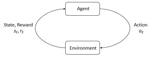
: Agent-Environment Interaction Loop

States and Observations

State $s$: complete description of the state of the world.
Observation $o$: partial description of a state.

Represent states and observations by:

real-valued vector (eg. the state of a robot can be represented by its joint angles and velocities)
matrix (eg. a visual state can be represented by the RGB matrix of its pixel values)
high-order tensor

Action Spaces

Discrete action spaces: only a finite number of moves are available to agent.
- Atari
- Go
Continuous action spaces: actions are real-valued vectors.
- Robot

Reward

The expression of reward: $r_t = R(s_t,a_t,s_{t+1})$.
Finite-horizon undiscounted return: $R(\tau) = \sum_{t=0}^T r_t$.
Infinite-horizon discounted return: $R(\tau) = \sum_{t=0}^{\infty} \gamma^t r_t$.

Policy

A policy is a rule used by an agent to decide what actions to take.

Parameterized policies: policies whose outputs are computable functions that depend on a set of parameters (the weights and biases of a neural network), which we can adjust to change the behavior via some optimization algorithm.

Deterministic policy: $a_t = \pi_\theta (s_t)$.

obs = tf.placeholder(shape=(None, obs_dim), dtype=tf.float32)
net = mlp(obs, hidden_dims=(64,64), activation=tf.tanh)
actions = tf.layers.dense(net, units=act_dim, activation=None)

Stochastic policy: $a_t \sim \pi_\theta (\cdot \vert s_t)$.
- Categorical policy:
  - Used in discrete action spaces.
  - Use softmax to convert the logits into probabilities $P_\theta(s)$.
  - Sampling: tf.distributions.Categorical.
  - Log-Likelihood: $\log \pi_\theta(a\vert s) = \log[P_\theta(s)]_a$.
- Diagonal Gaussian policy
  - Used in continuous action spaces.
  - A multivariate Gaussian distribution is described by a mean $\mu$ and a covariance matrix $\Sigma$.
  - The covariance matrix $\Sigma$ only has entries on the diagonal.
    1. $\log\sigma$ is not a function of state $s$, which are standalone parameters. (VPG, TRPO, PPO do it this way).
    2. There is a neural network that maps from states to log standard deviations $\log\sigma_\theta(s)$.
      - It may optionally share some layers with the mean network $\mu_\theta(s)$.
  - Output log standard deviations instead of standard deviations directly.
    - $\log\sigma \in(-\infty,\infty)$, while $\sigma \ge 0$.
    - It is easier to train parameters.
  - Sampling: $a = \mu_\theta(s) + \sigma_\theta(s)\odot N(0,I)$.
    - $\odot$ denotes the elementwise product of two vectors.
  - Log-Likelihood: $\log\pi_\theta(a\vert s) = -\frac{1}{2}\left( \sum_{i=1}^k \left( \frac{(a_i - \mu_i)^2}{\sigma_i^2} + 2\log\sigma_i \right) + k \log 2\pi \right)$.
    - $k$-dimensional action $a$.

Trajectories

A trajectory (also called episode or rollout):

\[\tau = (s_0,a_0,r_0,s_1,a_1,r_1, \cdots).\]

For finite horizon $t\in\{ 0,1,\cdots, T-1 \}$:

\[\tau = \{ (s_t,a_t,r_t) \}_{t=0}^{T-1} \cup \{ s_T \},\]

where the state trajectory is one step longer due to include the terminal state $s_T$, which for a non-infinite horizon has triggered some terminal condition.

Trajectories in the environment are subject to three different distributions:

The initial state distribution: $s_0 \sim \rho_0 (\cdot)$.
The state transition dynamics:
- Deterministic transition: $s_{s+1} = P(s_t,a_t)$.
- Stochastic transition: $s_{t+1} \sim P(\cdot \vert s_t,a_t)$.
The policy $\pi$.

Mathematical form of RL

Markov Decision Processes (MDPs): $\langle S,A,R,P,\rho_0,\gamma \rangle$.

$S$ is the set of all valid states.
$A$ is the set of all valid actions.
$R: S \times A \times S \to \mathbb{R}$ is the reward function, with $r_t = R(s_t,a_t,s_{s+1})$.
$P: S \times A \to P(S)$ is the transition probability function, with $P(s' \vert s,a)$.
$\rho_0$ is the starting state distribution.
$\gamma$ is the discount factor.

RL Optimization Problem

Optimization Objective

The goal of RL is to select a policy which maximizes expected reward when the agent acts according to it.

Suppose that both the environment transitions and the policy are stochastic, in this case, the probability of a T-step trajectory is:

\[P(\tau \vert \pi,P) = \rho_0(s_0) \prod_{t=0}^{T-1} P(s_{t+1} \vert s_t,a_t) \pi(a_t \vert s_t).\]

The expected reward is then:

\[J(\pi) = \int_{\tau} P(\tau \vert \pi,P) R(\tau) = \mathbb{E}_{\tau \sim \pi,P}[R(\tau)].\]

The central optimization objective in RL can be expressed by:

\[\pi^{\star} = \arg \max_{\pi} J(\pi).\]

Value and Action-Value Functions

On-Policy Value Function: the expected reward if you start in state $s$ and always act according to policy $\pi$:

\[V^{\pi}(s) = \mathbb{E}_{\tau \sim \pi,P} [R(\tau) \vert s_t = s] = \mathbb{E}_{\pi,P}[R_t\vert s_t = s].\]

On-Policy Action-Value Function: the expected reward if you start in state $s$, take an arbitrary action $a$ (may not come from the policy), and then forever after act according to policy $\pi$:

\[Q^{\pi}(s,a) = \mathbb{E}_{\tau \sim \pi,P} [R(\tau) \vert s_t = s, a_t = a] = \mathbb{E}_{\pi,P}[R_t\vert s_t =s,a_t =a].\]

Then, $V^\pi(s) = \mathbb{E}_{a\sim\pi}[Q^\pi(s,a)]$.

Optimal Value Function: always act according to the optimal policy in the environment:

\[V^{\star}(s) =\max_{\pi} \mathbb{E}_{\tau \sim \pi,P} [R(\tau) \vert s_t = s] = \max_a \mathbb{E}_P[R_t\vert s_t=s].\]

Optimal Action-Value Function:

\[Q^{\star}(s,a) =\max_{\pi} \mathbb{E}_{\tau \sim \pi,P} [R(\tau) \vert s_t = s, a_t = a] = \max_a \mathbb{E}_P[R_t\vert s_t=s,a_t=a].\]

Connections between the value function and the action-value function:

\[V^{\pi}(s) = \mathbb{E}_{a \sim \pi}[Q^{\pi}(s,a)],\] \[V^{\star}(s) = \max_a Q^{\star}(s,a).\]

Connection between the action-value function and the optimal action:

\[a^{\star}(s) = \arg \max_a Q^{\star}(s,a).\]

Advantage Function

减小方差，$V^\pi(s)$作为baseline

\[A^{\pi}(s,a) = Q^{\pi}(s,a) - V^{\pi}(s) = \mathbb{E}_P[r(s_t,a_t) + \gamma V^\pi(s_{t+1}) - V^\pi(s_t) \vert s_t =s,a_t=a].\]

Bellman Equations

\[\begin{aligned} V^\pi(s) & = \mathbb{E}_{\tau\sim\pi,P}[R(\tau)\vert s_t = s] \\ & = \mathbb{E}_{\pi,P}\left[ \sum_{k=0}^\infty \gamma^k r_{t+k+1} \big\vert s_t = s \right] \\ & = \mathbb{E}_{\pi,P}\left[ r_{t+1} + \gamma r_{t+2} + \gamma^2 r_{t+3} + \cdots \vert s_t = s \right] \\ & = \mathbb{E}_{\pi,P}\left[ r_{t+1} + \gamma \sum_{k=0}^\infty \gamma^k r_{t+k+2} \big\vert s_t = s \right] \\ & = \mathbb{E}_{(\pi,P)_t,(\pi,P)_{t+1}^\infty}\left[ r_{t+1} + \gamma \sum_{k=0}^\infty \gamma^k r_{t+k+2} \big\vert s_t = s \right] \\ & = \mathbb{E}_{(\pi,P)_t}\left[ \mathbb{E}_{(\pi,P)_{t+1}^\infty} [r_{t+1}\vert (\pi,P)_t] + \gamma \mathbb{E}_{\pi_{t+1}^\infty}\left[ \sum_{k=0}^\infty \gamma^k r_{t+k+2} \vert (\pi,P)_t \right] \big\vert s_t = s \right] \\ & = \mathbb{E}_{(\pi,P)_t}\left[ \mathbb{E}_{(\pi,P)_{t+1}^\infty} [r_{t+1}\vert a_t,s_{t+1}] + \gamma \mathbb{E}_{(\pi,P)_{t+1}^\infty}\left[ \sum_{k=0}^\infty \gamma^k r_{t+k+2} \vert a_t,s_{t+1} \right] \big\vert s_t = s \right] \\ & = \mathbb{E}_{(\pi,P)_t}\left[ \mathbb{E}_{(\pi,P)_{t+1}^\infty} [r_{t+1}\vert a_t,s_{t+1}] + \gamma \mathbb{E}_{(\pi,P)_{t+1}^\infty}\left[ \sum_{k=0}^\infty \gamma^k r_{t+k+2} \vert s_{t+1} \right] \big\vert s_t = s \right] \\ & = \mathbb{E}_{(\pi,P)_t}\left[ r_{t+1} + \gamma V^\pi(s_{t+1}) \vert s_t = s \right] \\ & = \mathbb{E}_{a\sim\pi,s'\sim P}[r(s,a) + \gamma V^\pi(s')]. \end{aligned}\]

Where

$\pi,P = (\pi,P)_t^\infty = (\pi,P)_t,(\pi,P)_{t+1}^\infty$.
$(\pi,P)_t := a_t\sim\pi(\cdot\vert s_t), s_{t+1}\sim P(s_t,a_t) = (a_t,s_{t+1})$.
$\mathbb{E}_{\pi,P}[\cdot] = \mathbb{E}_{(\pi,P)_t,(\pi,P)_{t+1}^\infty}[\cdot] = \mathbb{E}_{(\pi,P)_t}[\mathbb{E}_{(\pi,P)_{t+1}^\infty}[\cdot\vert (\pi,P)_t]]$.
- For a joint probability distribution $p(x,y) = p(x)p(y\vert x)$, then, $\mathbb{E}_{x,y\sim p(x,y)}[\cdot] = \mathbb{E}_{x\sim p(x)}[\mathbb{E}_{y\sim p(y\vert x)}[\cdot]]$, also can be written as $\mathbb{E}_{x,y}[\cdot] = \mathbb{E}_x[\mathbb{E}_y[\cdot\vert x]]$.
$r_{t+1}$ is the reward between $t$ and $t+1$ timestep, which is independent of $(\pi,P)_{t+1}^\infty$, then, $\mathbb{E}_{(\pi,P)_{t+1}^\infty}[r_{t+1}\vert (\pi,P)_t] = r_{t+1}$.
$(\pi,P)_{t+1}^\infty$ is independent of $a_t$, and only related to $s_{t+1}$, thus, $\mathbb{E}_{(\pi,P)_{t+1}^\infty}\left[ \sum_{k=0}^\infty \gamma^k r_{t+k+2} \vert a_t,s_{t+1} \right] = \mathbb{E}_{(\pi,P)_{t+1}^\infty}\left[ \sum_{k=0}^\infty \gamma^k r_{t+k+2} \vert s_{t+1} \right] = V^\pi(s_{t+1})$.

Therefore, the Bellman equations for $V^\pi$ and $Q^\pi$ are:

\[V^{\pi}(s) = \mathbb{E}_{a \sim \pi, s' \sim P}[r(s,a) + \gamma V^{\pi}(s')],\] \[Q^{\pi}(s,a) = \mathbb{E}_{s' \sim P}\left[ r(s,a) + \gamma \mathbb{E}_{a' \sim \pi} [Q^{\pi}(s',a')] \right].\]

Bellman Optimality Equations

\[V^{\star}(s) =\max_a \mathbb{E}_{s' \sim P}[r(s,a) + \gamma V^{\star}(s')] = \max_a \sum_{s'}p(s' \vert s,a)[r(s,a) + \gamma V^{\star}(s')],\] \[Q^{\star}(s,a) = \mathbb{E}_{s' \sim P}\left[ r(s,a) + \gamma \max_{a'} Q^{\star}(s',a') \right] = \sum_{s'}p(s' \vert s,a) \left[ r(s,a) + \gamma \max_{a'} Q^{\star}(s',a') \right].\]

Bellman Backup Operator

定义

定义Bellman backup算子$\mathcal{T}^\pi$(关于$Q$的操作函数)：

\[[\mathcal{T}^\pi Q](s_t,a_t) = \mathbb{E}_P[r_t + \gamma\mathbb{E}_{a_{t+1}\sim\pi}[Q(s_{t+1}, a_{t+1})]].\]

Bellman backup算子就是把Bellman等式中的$Q^\pi$替换为被作用的$Q$函数。
$Q^\pi$就是该算子的不动点，即$\mathcal{T}^\pi Q^\pi = Q^\pi$.
对任意$Q$作用无限多次$\mathcal{T}^\pi$可以收敛到$Q^\pi$.
- $Q, \mathcal{T}^\pi Q, (\mathcal{T}^\pi)^2 Q, \cdots \to Q^\pi$.

\[[\mathcal{T} Q](s_t,a_t) = \mathbb{E}_P\left[ t_t + \gamma\max_{a_{t+1}}Q(s_{t+1},a_{t+1}) \right].\]

基于采样的估计

\[[\widehat{\mathcal{T}Q}](s_t,a_t) = r_t + \gamma \max_{a_{t+1}}Q(s_{t+1,a_{t+1}}).\] \[[\widehat{\mathcal{T}^\pi Q}](s_t,a_t) = r_t + \gamma \mathbb{E}_P[Q(s_{t+1,a_{t+1}})].\]

References:

RL Optimization Algorithms

: A Taxonomy of RL Algorithms

Model-Free vs Model-Based RL

Whether the agent has access to (or learn) a model of the environment?

Model of the environment: means that a function which predicts state transitions and rewards.

The main upside to having a model is that it allows the agent to plan by thinking ahead, seeing what would happen for a range of possible choices and explicitly deciding between its options. When this works, it can result in a substantial improvement in sample efficiency over methods that don’t have a model.

The main downside is that a ground-truth model of the environment is usually not available to the agent. Therefore, the agent has to learn the model purely from experience. The biggest challenge is that bias in the model can be exploited by the agent, resulting in an agent which performs well w.r.t. the learned model, but behaves sub-optimally in the real environment.

What to Learn?

Policy
- stochastic policy
- deterministic policy
Value function
- value function
- action-value function (Q-function)
Model of environment
- stochastic model
- deterministic model

What to Learn in Model-Free RL

There are two main approaches to representing and training agents with model-free RL:

Policy Optimization: represent a policy explicitly as $\pi_\theta(a \vert s)$, and optimize the parameters $\theta$ by gradient descent on the performance objective $J(\pi_\theta)$, or indirectly, by maximizing local approximations of $J(\pi_\theta)$.
Q-Learning: learn an approximator $Q_\theta(s,a)$ for the optimal action-value function $Q^{\star}(s,a)$. They use an objective function based on Bellman equation, and the optimization is almost performed off-policy, which means that each update can use data collected at any point during training.

What to Learn in Model-Based RL

Pure Planning: use model predictive control (MPC) to select actions w.r.t. the model.
Expert Iteration: learning an explicit representation of the policy $\pi_\theta(a \vert s)$, the agent uses a planning algorithm in the model to generate candidate actions, which is better than what the policy alone would have produced.
Data Augmentation for Model-Free Methods: augment real experiences with fictitious ones in updating the agent or use only fictitious experiences for updating the agent, which is called “training in the dream”.
Embeddig Planning Loops into Policies: the policy can learn to choose how and when to use the plans, this makes model bias less of a problem, because if the model is bad for planning in some states, the policy can simply learn to ignore it.