An Overview of Gradient Descent Algorithms
Once we have the model of our Neural Network, we need to find the best set of parameters to minimize the training/test loss and maximize the accuracy of the model.
Model solver brings together training data, the model and the optimization algorithms to train the model. A model solver has:
- Training and Test dataset
- Reference to the model
- Different type of
optimizerslike SGD, Adam \(\cdots\) - Record the loss and accuracy for the training phase of each epoch
- Optimized parameters for the model
Thanks to active research, we are much better equipped with various optimization algorithms than just Vanilla Gradient Descent. Let us start developing the ideas around building the model solver and discuss the different approaches to Gradient Descent (SGD, Momentum, NAG, AdaGrad, RMSprop, Adam).
Gradient Descent is the most common optimization algorithm used in Machine Learning. It uses gradient of loss function to find the global minima by taking one step at a time toward the negative of the gradient.
Why Gradient Descent?
Gradient Descent along with Backpropagation algorithm has become the de-facto learning algorithm of Neural Networks.
Newton's Method, we need to calculate second order partial derivative matrix or Hessian matrix. Although the algorithm makes efficient updates and doesn’t require learning rate parameter, we have to calculate second order partial derivatives matrix for every parameter w.r.t. every other parameter, which makes it very computationally costly and highly ineffective in terms of memory.
Gradient Descent requires only first order deritives of parameters w.r.t. the loss function, which is efficiently calculated by Backpropagation, and so it shines above these techniques because of its simplicity and efficiency.
Stochastic Gradient Descent (SGD)
When training input is very large, gradient descent (GD) is quite slow to converge. SGD is the preferred variation of GD which estimates the gradient from a small sample of randomly chosen training input in each iteration called minibatches.
Minibatches
Minibatches are generated by shuffling the training data and randomly selecting certain number of training samples. This number of samples is called minibatch size and is a parameter to SGD. Here is the code:
def get_minibatches(X,y,minibatch_size):
    m = X.shape[0]
    minibatches = []
    X,y = shuffle(X,y)
    for i in range (0,m,minibatch_size):
        X_batch = X[i:i+minibatch_size,:,:,:]
        y_batch = y[i:i+minibatch_size,]
        minibatches.append((X_batch,y_batch))
    return minibatches
Update Rule
SGD uses a very simple update rule to change the parameters along the negative gradient.
Mathematically,
\[w = w - \alpha \nabla_w L (w;x^{(i:i+n)};y^{(i:i+n)}),\]where \(n\) denotes the minibatch size.
params: a list learnable parameters for each layer.
grads: a similar list for gradients.
Here is the code:
def vanilla_update(params,grads,learning_rate=0.01):
    for param,grad in zip(params,reversed(grads)): # grads are in opposite order of params
        for i in range(len(grad)):
            param[i] += - learning_rate * grad[i]
SGD Algorithm
epoch: every complete exposure of the training dataset.
The algorithm code:
def sgd(nnet,X_train,y_train,minibatch_size,epoch,learning_rate,verbose=True,X_test=None,y_test=None):
    minibatches = get_minibatches(X_train,y_train,minibatch_size)
    for i in range(epoch):
        loss = 0
        if verbose:
            print("Epoch {0}".format(i+1))
        for X_mini, y_mini in minibatches:
            loss,grads = nnet.train_step(X_mini,y_mini)
            vanilla_update(nnet.params,grads,learning_rate = learning_rate)
        if verbose:
            train_acc = accuracy(y_train,nnet.predict(X_train))
            test_acc = accuracy(y_test,nnet.predict(X_test))
            print("Loss = {0} | Training Accuracy = {1} | Test Accuracy = {2}".format(loss,train_acc,test_acc))
    return nnet
SGD with Momentum
Momentum technique is an approach which provides an update rule that is motivated from the physical perspective of optimization. Imagine a ball in a hilly terrain is trying to reach the deepest valley. when the slope of the hill is very high, the ball gains a lot of momentum and is able to pass through slight hills in its way. As the slope decreases the momentum and speed of the ball decreases, eventually coming to rest in the deepest position of valley.
This technique modifies the standard SGD by introducing velocity \(v\), which is the parameter we are trying to optimize, and friction \(\mu\), which tries to control the velocity and prevents overshooting the valley while allowing faster descent. The gradient only has direct influence on the velocity, which in turn has an effect on the position.
Mathematically,
\[v_t = \mu v_{t-1} + \alpha \nabla_w L (w),\] \[w = w - v_t.\]Which translates to code as:
def momentum_update(velocity,params,grads,learning_rate=0.01,mu=0.9):
    for v,param,grad, in zip(velocity,params,reversed(grads)):
        for i in range(len(grad)):
            v[i] = mu*v[i] + learning_rate * grad[i]
            param[i] -= v[i]
Advantage: makes very small change to SGD but provides a big boost to speed of learning.
SGD with Momentum Update Rule
We need to store the velocity for all the parameters, and use this velocity for making the updates. Here is the code:
def sgd_momentum(nnet,X_train,y_train,minibatch_size,epoch,learning_rate,mu = 0.9,verbose=True,X_test=None,y_test=None):
    minibatches = get_minibatches(X_train,y_train,minibatch_size)
    for i in range(epoch):
        loss = 0
        velocity = []
        for param_layer in nnet.params:
            p = [np.zeros_like(param) for param in list(param_layer)]
            velocity.append(p)

        if verbose:
            print("Epoch {0}".format(i+1))
        for X_mini, y_mini in minibatches:
            loss,grads = nnet.train_step(X_mini,y_mini)
            momentum_update(velocity,nnet.params,grads,learning_rate=learning_rate,mu=mu)

        if verbose:
            train_acc = accuracy(y_train,nnet.predict(X_train))
            test_acc = accuracy(y_test,nnet.predict(X_test))
            print("Loss = {0} | Training Accuracy = {1} | Test Accuracy = {2}".format(loss,train_acc,test_acc))
    return nnet
Nesterov Accelerated Gradient (NAG)
NAG is a clever variation of momentum that works slightly better than standard Momentum.
Idea: instead of calculating the gradient at current position, we calculate the gradient at a positon that we know our momentum is about to take us, called as "look ahead" positon. From physical perspective, it makes sense to make judgements about our final position based on the position that we know we are going to be in a short while.
The implementation makes a slight modeification to standard SGD with Momentum by nudging our parameters slightly in the direction of the velocity and calculating the gradient there.
Mathematically,
\[v_t = \mu v_{t-1} + \alpha \nabla_w L (w - \mu v_{t-1}),\] \[w = w - v_t.\]Here is the code:
def sgd_momentum(nnet,X_train,y_train,minibatch_size,epoch,learning_rate,mu = 0.9,verbose=True,X_test=None,y_test=None,nesterov = False):

    minibatches = get_minibatches(X_train,y_train,minibatch_size)

    for i in range(epoch):
        loss = 0
        velocity = []
        for param_layer in nnet.params:
            p = [np.zeros_like(param) for param in list(param_layer)]
            velocity.append(p)

        if verbose:
            print("Epoch {0}".format(i+1))

        for X_mini, y_mini in minibatches:
            # if nesterov is enabled, nudge the params forward by momentum
            # to calculate the gradients in a "look ahead" position
            if nesterov:
                for param,ve in zip(nnet.params,velocity):
                    for i in range(len(param)):
                        param[i] += mu*ve[i]

            loss,grads = nnet.train_step(X_mini,y_mini)
            momentum_update(velocity,nnet.params,grads,learning_rate=learning_rate,mu=mu)

        if verbose:
            train_acc = accuracy(y_train,nnet.predict(X_train))
            test_acc = accuracy(y_test,nnet.predict(X_test))
            print("Loss = {0} | Training Accuracy = {1} | Test Accuracy = {2}".format(loss,train_acc,test_acc))
    return nnet
Until now, we have used a global and equal learning rate for all our parameters. So all of our parameters are being updated with constant factor. But what if we could speed up or slow down this factor, even for each parameter, as the training progresses?
We could adaptively tune the learning throughout the training phases and know which direction to accelerate and which to decelerate. Several methods that use such adaptive learning rates have been proposed, most notably AdaGrad, RMSprop and Adam.
Adaptive Gradient (AdaGrad)
AdaGrad keeps track of per parameter sum of squared gradient and normalizes parameter update step.
Idea: parameters which receive big updates will have their effective learning rate reduced, while parameters which receive small updates will have their effective learning rate increased. This way we can accelerate the convergence by accelerating per parameter learning.
Mathematically,
\[g_{t,i} = \nabla_{w_t} L (w_{t,i}),\] \[w_{t+1,i} = w_{t,i} - \frac{\alpha}{\sqrt{G_{t,ii}} + \epsilon} g_{t,i}.\]The code:
def adagrad_update(cache,params,grads,learning_rate=0.01):
    for c,param,grad, in zip(cache,params,reversed(grads)):
        for i in range(len(grad)):
            cache[i] += grad[i]**2
            param[i] += - learning_rate * grad[i] / (np.sqrt(cache[i])+1e-8) # for preventing divide by 0
Disadvantage: cache[i] += grad[i]**2 the update is monotonically increasing. This can pose problems because the learning rate can steadily decrease to the point where it stops the learning altogether.
RMSprop
RMSprop combats the above problem by decaying the past squared gradient via a factor decay_rate to control the aggressive learning rates.
Mathematically,
\[E [g^2]_t = d E [g^2]_{t-1} + (1 - d) g_t^2,\] \[w_{t+1} = w_t - \frac{\alpha}{\sqrt{E [g^2]_t} + \epsilon} g_t,\]where \(d\) denotes the factor decay_rate which is a hyperparameter with typical values like 0.9, 0.99 and so on.
The code:
def rmsprop_update(cache,params,grads,learning_rate=0.01,decay_rate=0.9):
    for c,param,grad, in zip(cache,params,reversed(grads)):
        for i in range(len(grad)):
            cache[i] = decay_rate * cache[i] + (1-decay_rate) * grad[i]**2
            param[i] += - learning_rate * grad[i] / (np.sqrt(cache[i])+1e-4)
Adaptive Moment Estimation (Adam)
Adam is another method that computes adaptive learning rates for each parameter. In addition to storing an exponentially decaying average of past squared gradients \(n_t\) like RMSprop, Adam also keeps an exponentially decaying average of past gradients \(c_t\).
\[c_t = \beta_1 c_{t-1} + (1 - \beta_1) g_t,\] \[n_t = \beta_2 n_{t-1} + (1 - \beta_2) g_t^2.\]Another thing to note is that Adam includes bias correction mechanism, which compensates for first few iterations when both \(c_t\) and \(n_t\) are biasd at zero as they are initialized to zero. We will here derive the term for the second moment estimate, the derivation for the first moment estimate is completely analogous. We can write the second moment estimate as a function of the gradients at all previous timesteps:
Then, we can compare the expected value of the exponential moving average \(E [n_t]\) at timestep \(t\) with the true second moment \(E [g_t^2]\), so we can correct for the discrepancy between the two values.
\[\begin{align} E [n_t] & = E \left[ (1 - \beta_2) \sum_{i=1}^t \beta_2^{t-i} g_i^2 \right] \\ & = E [g_t^2] (1 - \beta_2) \sum_{i=1}^t \beta_2^{t-i} + \zeta \\ & = E [g_t^2] (1 - \beta_2^t) + \zeta. \end{align}\]What is left is the term \((1 - \beta_2^t)\) which is caused by initializing the running average with zeros. We therefore divide by this term to correct the initialization bias:
\[\hat{c_t} = \frac{c_t}{1 - \beta_1^t},\] \[\hat{n_t} = \frac{n_t}{1 - \beta_2^t},\] \[w_{t+1} = w_t - \frac{\alpha}{\sqrt{\hat{n_t}} + \epsilon} \hat{c_t}.\]The implementation of Adam:
def adam(nnet,X_train,y_train,minibatch_size,epoch,learning_rate,verbose=True,X_test=None,y_test=None,beta1=0.9,beta2=0.999):

    minibatches = get_minibatches(X_train,y_train,minibatch_size)
    for i in range(epoch):
        loss = 0
        velocity,cache = [],[]
        for param_layer in nnet.params:
            p = [np.zeros_like(param) for param in list(param_layer)]
            velocity.append(p)
            cache.append(p)
        if verbose:
            print("Epoch {0}".format(i+1))
        t = 1
        for X_mini, y_mini in minibatches:
            loss,grads = nnet.train_step(X_mini,y_mini)
            for c,v,param,grad, in zip(cache,velocity,nnet.params,reversed(grads)):
                for i in range(len(grad)):
                    c[i] = beta1 * c[i] + (1-beta1) * grad[i]
                    mt = c[i] / (1 - beta1**t)
                    v[i] = beta2 * v[i] + (1-beta2) * (grad[i]**2)
                    vt = v[i] / (1 - beta2**t)
                    print(vt)
                    param[i] += - learning_rate * mt / (np.sqrt(vt) + 1e-4)
            t+=1

        if verbose:
            train_acc = accuracy(y_train,nnet.predict(X_train))
            test_acc = accuracy(y_test,nnet.predict(X_test))
            print("Loss = {0} | Training Accuracy = {1} | Test Accuracy = {2}".format(loss,train_acc,test_acc))
    return nnet
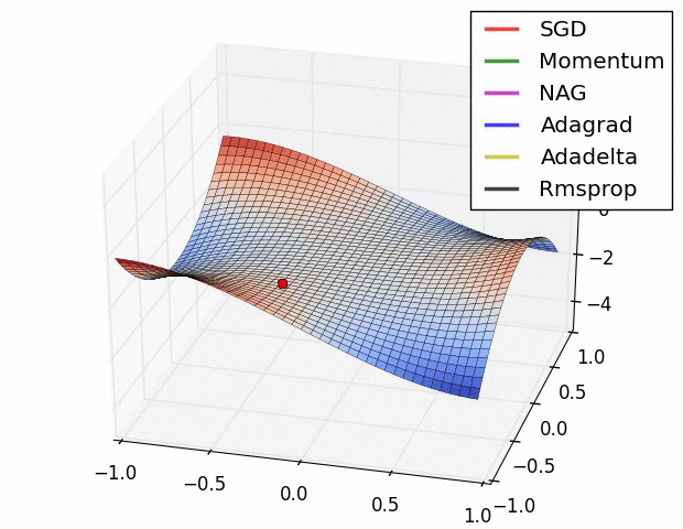
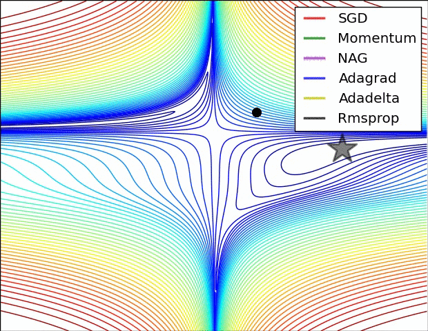
We can contrast the gradient descent algorithms by the following pictures:
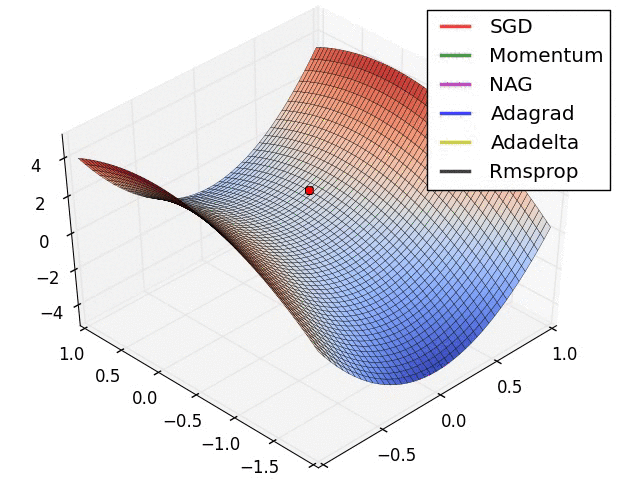
- Long Valley
- Saddle Point
- Beale's Function