Implementation of CNN by Numpy
Understand the concepts and mathematics behind Convolutional Neural Network (CNN) and implement the CNN by Numpy in Python.
Convolution Layer
- Convolutional Operation
Convolutional operation takes a patch of the image, and applies a filter by performing a dot product on it.
The input volume of the convolution layer:
- \(N\): Number of input
- \(C\): Depth of input
- \(H\): Height of input
- \(W\): Width of input
The hyperparameters of the convolutional operation:
- \(K\): Number of filters
- \(F\): Spatial extent
- \(S\): Stride length
- \(P\): Zero padding
Then, the spatial size of output is \([(H-F+2P)/S+1] * [(W-F+2P)/S+1]\).
Forward Propagation
- Forward-Backward Propagation
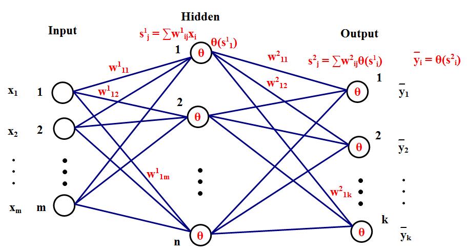
Convolution layer replaces the matrix multiplication with convolutional operation. To compute the nolinear input for \(j^{th}\) neuron on \(l\) layer, we have:
\[S_j^l = \sum W_{ij}^l \theta (S_i^{l-1}) + b_j^l.\]We loop over each image, each channel and take a dot product at each \(F*F\) location for each of our filters to do the convolutional operation. Lets examine this with a simple example.
Suppose we have a single image of size \(1*1*4*4\) and a single filter \(1*1*2*2\) and use \(S=1\) and \(P=1\). Then,
\[X = \begin{bmatrix} 0 & 1 & 2 & 3 \\ 4 & 5 & 6 & 7 \\ 8 & 9 & 10 & 11 \\ 12 & 13 & 14 & 15 \end{bmatrix}_{4 \times 4},\] \[X_{pad} = \begin{bmatrix} 0 & 0 & 0 & 0 & 0 & 0 \\ 0 & 0 & 1 & 2 & 3 & 0 \\ 0 & 4 & 5 & 6 & 7 & 0 \\ 0 & 8 & 9 & 10 & 11 & 0 \\ 0 & 12 & 13 & 14 & 15 & 0 \\ 0 & 0 & 0 & 0 & 0 & 0 \end{bmatrix}_{6 \times 6}.\]Then, we have \((4-2+2*1)/1+1 = 5\) locations along both width and height, so 25 locations to do our convolution. For each location, we stretch out to \(4*1\) column vector. Thus, we have 25 of these column vertors and the matrix of all the stretched out receptive fields \(X_{col}\) which size is \(4 * 25\).
If we have 3 filters of size \(1*2*2\) then we have weights matrix \(W_{row}\) of size \(3 * 4\).
The result of convolution is now equivalent of performing a single matrix multiplication np.dot(W_row, X_col) which has the dot product of every filter with every receptive field. The result matrix \(3*25\) which can be reshaped back to get output volume of size \(1*3*5*5\).
We use im2col utility to perform the reshaping of input \(X\) to \(X_{col}\).
Here is the code:
# Create a matrix of size (h_filter*w_filter) by n_X * ((h_X-h_filter+2p)/stride + 1)**2
# suppose X is 5x3x10x10 with 3x3x3 filter and padding and stride = 1
# X_col will be 27x500
X_col = im2col_indices(X,h_filter,w_filter,padding,stride)
# suppose we have 10 filter of size 10x3x3x3, W_col will be 10x27
W_col = W.reshape(n_filter,c_filter*h_filter*w_filter)
# output will be 10x500
output = np.dot(W_col,X_col) + b
# reshape to get 10x10x10x5 and then transpose the axes 5x10x10x10
output = output.reshape(n_filter,h_out,w_out,n_X).transpose(3,0,1,2)
Backward Propagation
- Weights Update
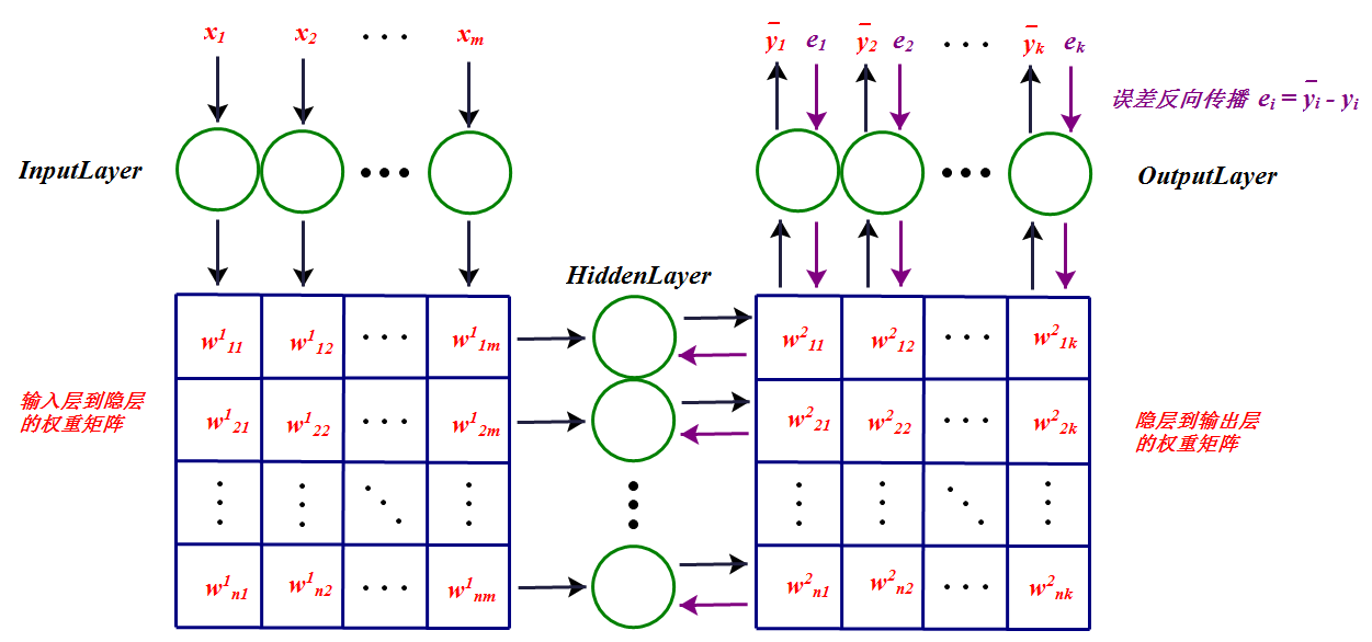
Define the loss function as RMSE:
\[L(e) = \frac{1}{2} \sum_{j=0}^{k} e_j^2 = \frac{1}{2} \sum_{j=0}^{k} (\bar{y_j} - y_j)^2.\]Then, we need to minimize the loss function to obtain the accurate values of weights at each layer. The common method used is gradient descent algorithm. The gradient of each layer can be obtained as follows:
\[\frac{\partial L}{\partial w_{ij}^1} = \frac{\partial L}{\partial s_j^1} \frac{\partial s_j^1}{\partial w_{ij}^1},\] \[\frac{\partial L}{\partial b_j^1} = \frac{\partial L}{\partial s_j^1} \frac{\partial s_j^1}{\partial b_j^1},\] \[s_j^1 = \sum_{i=1}^m x_i w_{ij}^1 + b_j^1,\] \[\frac{\partial s_j^1}{\partial w_{ij}^1} = x_i,\] \[\frac{\partial s_j^1}{\partial b_j^1} = 1,\] \[\frac{\partial L}{\partial w_{ij}^1} = \frac{\partial L}{\partial s_j^1} x_i,\] \[\frac{\partial L}{\partial b_j^1} = \frac{\partial L}{\partial s_j^1}.\]Then, we need to calculate \(\frac{\partial L}{\partial s_j^1}\).
\[\frac{\partial L}{\partial s_j^1} = \sum_{i=1}^k \frac{\partial L}{\partial s_i^2} \frac{\partial s_i^2}{\partial s_j^1},\] \[s_i^2 = \sum_{j=0}^n \theta (s_j^1) w_{ji}^2 + b_i^2,\] \[\frac{\partial s_i^2}{\partial s_j^1} = \frac{\partial s_i^2}{\partial \theta (s_j^1)} \frac{\partial \theta (s_j^1)}{\partial s_j^1} = w_{ji}^2 \theta' (s_j^1),\] \[\frac{\partial L}{\partial s_j^1} = \sum_{i=1}^k \frac{\partial L}{\partial s_i^2} w_{ji}^2 \theta' (s_j^1) = \theta' (s_j^1) \sum_{i=1}^k \frac{\partial L}{\partial s_i^2} w_{ji}^2.\]Let \(\delta_i^l = \frac{\partial L}{\partial s_i^l}\),
\[\delta_j^1 = \theta' (s_j^1) \sum_{i=1}^k \delta_i^2 w_{ji}^2,\] \[\delta_i^2 = \frac{\partial L}{\partial s_i^2} = \frac{\partial \sum_{j=0}^k \frac{1}{2} (\bar{y_j} - y_j)^2}{\partial s_i^2} = (\bar{y_i} - y_i) \frac{\partial \bar{y_i}}{\partial s_i^2} = e_i \frac{\partial \bar{y_i}}{\partial s_i^2} = e_i \theta' (s_i^2).\]Thus,
\[\frac{\partial L}{\partial w_{ij}^1} = \delta_j^1 x_i,\] \[\frac{\partial L}{\partial b_j^1} = \delta_j^1,\] \[\frac{\partial L}{\partial w_{ij}^2} = \frac{\partial L}{\partial s_j^2} \frac{\partial s_j^2}{\partial w_{ij}^2} = \delta_j^2 \theta(s_i^1),\] \[\frac{\partial L}{\partial b_j^2} = \frac{\partial L}{\partial s_j^2} \frac{\partial s_j^2}{\partial b_j^2} = \delta_j^2.\]We can see the internal of a single neuron:
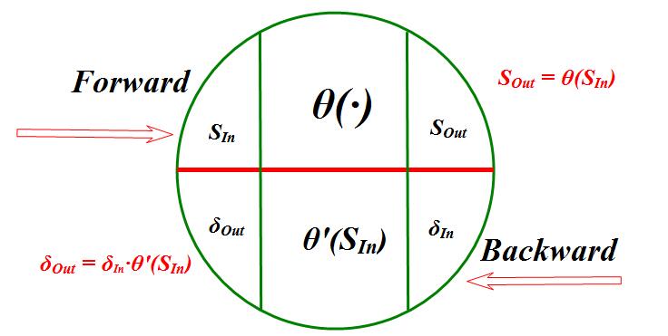
- Internal operation of neuron
Here is the code:
# from 5x10x10x10 to 10x10x10x5 and 10x500
dout_flat = dout.transpose(1,2,3,0).reshape(n_filter,-1)
# calculate dot product 10x500 . 500x27 = 10x27
dW = np.dot(dout_flat,X_col.T)
# reshape back to 10x3x3x3
dW = dW.reshape(W.shape)
# for bias gradient
db = np.sum(dout,axis=(0,2,3))
db = db.reshape(n_filter,-1)
# from 10x3x3x3 to 10x9
W_flat = W.reshape(n_filter,-1)
# dot product 9x10 . 10x500 = 9x500
dX_col = np.dot(W_flat.T,dout_flat)
# get the gradients for real image from the stretched image.
# from the stretched out image to real image i.e. 9x500 to 5x3x10x10
dX = col2im_indices(dX_col,X.shape,h_filter,w_filter,padding,stride)
Source Code
Here is the source code for Convolution Layer with forward and backward API implemented:
class Conv():

    def __init__(self, X_dim, n_filter, h_filter, w_filter, stride, padding):

        self.d_X, self.h_X, self.w_X = X_dim

        self.n_filter, self.h_filter, self.w_filter = n_filter, h_filter, w_filter
        self.stride, self.padding = stride, padding

        self.W = np.random.randn(n_filter, self.d_X, h_filter, w_filter) / np.sqrt(n_filter / 2.)
        self.b = np.zeros((self.n_filter, 1))
        self.params = [self.W, self.b]

        self.h_out = (self.h_X - h_filter + 2 * padding) / stride + 1
        self.w_out = (self.w_X - w_filter + 2 * padding) / stride + 1

        if not self.h_out.is_integer() or not self.w_out.is_integer():
            raise Exception("Invalid dimensions!")

        self.h_out, self.w_out = int(self.h_out), int(self.w_out)
        self.out_dim = (self.n_filter, self.h_out, self.w_out)

    def forward(self, X):

        self.n_X = X.shape[0]

        self.X_col = im2col_indices(X, self.h_filter, self.w_filter, stride=self.stride, padding=self.padding)
        W_row = self.W.reshape(self.n_filter, -1)

        out = W_row @ self.X_col + self.b
        out = out.reshape(self.n_filter, self.h_out, self.w_out, self.n_X)
        out = out.transpose(3, 0, 1, 2)
        return out

    def backward(self, dout):

        dout_flat = dout.transpose(1, 2, 3, 0).reshape(self.n_filter, -1)

        dW = dout_flat @ self.X_col.T
        dW = dW.reshape(self.W.shape)

        db = np.sum(dout, axis=(0, 2, 3)).reshape(self.n_filter, -1)

        W_flat = self.W.reshape(self.n_filter, -1)

        dX_col = W_flat.T @ dout_flat
        shape = (self.n_X, self.d_X, self.h_X, self.w_X)
        dX = col2im_indices(dX_col, shape, self.h_filter, self.w_filter, self.padding, self.stride)

        return dX, [dW, db]
Pooling Layer
- Max-pooling
The pooling layer is usually placed after the convolution layer. The utility of pooling layer is to reduce the spatial dimension of the input volume for next layers. It only affects width and height but not depth.
The input size of the pooling layer: \(W_1 * H_1 * D_1\).
The hyperparameters used are:
- \(F\): Spatial extent
- \(S\): Stride length
The output size is \(W_2 * H_2 * D_2\), where \(W_2 = (W_1-F)/S + 1\), \(H_2 = (H_1-F)/S + 1\), \(D_2 = D_1\).
Note: There are no learnable parameters and it is not common to use zero padding in pooling layer.
Forward Propagation
Similar to doing convolution operation in convolution layer, we select the max values in the receptive fields of the input in the max-pooling layer, and save the indices and then produce a summarized output volume. The implementation of the forward pass is as follows:
# convert channels to separate images so that im2col can arrange them into separate column
X_reshaped = X.reshape(n_X * c_X, 1, h_X, w_X)
X_col = im2col_indices(X_reshaped,h_filter,w_filter,padding = 0,stride = stride)
# find the max index in each receptive field
max_idx = np.argmax(X_col,axis=0)
out = X_col[max_idx, range(max_idx.size)]
# reshape and re-organize the output
out = out.reshape(h_out,w_out,n_X,c_X).transpose(2,3,0,1)
Backward Propagation
For the backward pass of the gradient, we start with a zero matrix and fill the max index of the matrix with the gradient from above. The reason behind this is that there is no gradient for non max neurons, as changing them slightly doesn't change the output. So gradient from the next layer is passed only to the neurons that achieved max, and all the other neurons get zero gradient.
dX_col = np.zeros_like(X_col)
# flatten dout so that we can index using max_idx from forward pass
dout_flat = dout.transpose(2,3,0,1).ravel()
# now fill max index with the gradient
dX_col[max_idx,range(max_idx.size)] = dout_flat
Since we stretch out the images to columns in the forward pass, we revert this action before we pass back the input gradient.
# convert stretched image to real image
dX = col2im(dX_col,X_reshaped.shape,h_filter,w_filter,padding = 0, stride=stride)
dX = dX.reshape(X.shape)
Source Code
Here is the source code for Maxpool Layer with forward and backward API implemented:
class Maxpool():

    def __init__(self, X_dim, size, stride):

        self.d_X, self.h_X, self.w_X = X_dim

        self.params = []

        self.size = size
        self.stride = stride

        self.h_out = (self.h_X - size) / stride + 1
        self.w_out = (self.w_X - size) / stride + 1

        if not self.h_out.is_integer() or not self.w_out.is_integer():
            raise Exception("Invalid dimensions!")

        self.h_out, self.w_out = int(self.h_out), int(self.w_out)
        self.out_dim = (self.d_X, self.h_out, self.w_out)

    def forward(self, X):
        self.n_X = X.shape[0]
        X_reshaped = X.reshape(X.shape[0] * X.shape[1], 1, X.shape[2], X.shape[3])

        self.X_col = im2col_indices(X_reshaped, self.size, self.size, padding=0, stride=self.stride)

        self.max_indexes = np.argmax(self.X_col, axis=0)
        out = self.X_col[self.max_indexes, range(self.max_indexes.size)]

        out = out.reshape(self.h_out, self.w_out, self.n_X, self.d_X).transpose(2, 3, 0, 1)
        return out

    def backward(self, dout):

        dX_col = np.zeros_like(self.X_col)
        # flatten the gradient
        dout_flat = dout.transpose(2, 3, 0, 1).ravel()

        dX_col[self.max_indexes, range(self.max_indexes.size)] = dout_flat

        # get the original X_reshaped structure from col2im
        shape = (self.n_X * self.d_X, 1, self.h_X, self.w_X)
        dX = col2im_indices(dX_col, shape, self.size, self.size, padding=0, stride=self.stride)
        dX = dX.reshape(self.n_X, self.d_X, self.h_X, self.w_X)
        return dX, []
Activation Functions
Activation function is the mapping between the output of last layer and the input of next layer.
Why need activation function?
If there is non activation function used (equivaliently, the activation function is \(f(x) = x\)), the input of next layer will equal to the output of last layer. Thus, the output of the CNN will always be the linear combination of the input. This will limit the approximation capability of the CNN. So, we use the nonlinear function as the activation function to improve the performance of CNN.
Rectified Linear Units (ReLU)
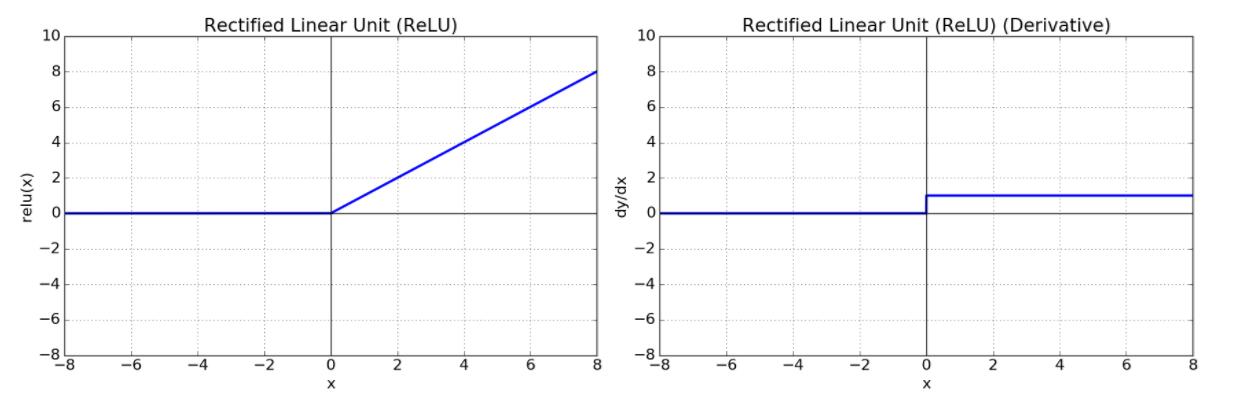
- ReLU
Here is the code:
class ReLU():
    def __init__(self):
        self.params = []

    def forward(self, X):
        self.X = X
        return np.maximum(0, X)

    def backward(self, dout):
        dX = dout.copy()
        dX[self.X <= 0] = 0
        return dX, []
Sigmoid
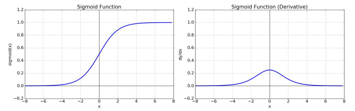
- Sigmoid
Here is the code:
class sigmoid():
    def __init__(self):
        self.params = []

    def forward(self, X):
        out = 1.0 / (1.0 + np.exp(X))
        self.out = out
        return out

    def backward(self, dout):
        dX = dout * self.out * (1 - self.out)
        return dX, []
Hyperbolic Tangent Function (tanh)
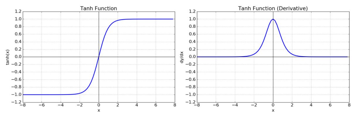
- tanh
Here is the code:
class tanh():
    def __init__(self):
        self.params = []

    def forward(self, X):
        out = np.tanh(X)
        self.out = out
        return out

    def backward(self, dout):
        dX = dout * (1 - self.out**2)
        return dX, []
Gaussian Function
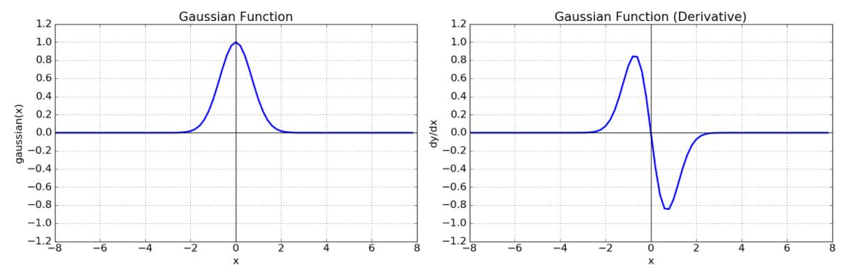
- Gaussian
Fully Connected Layer
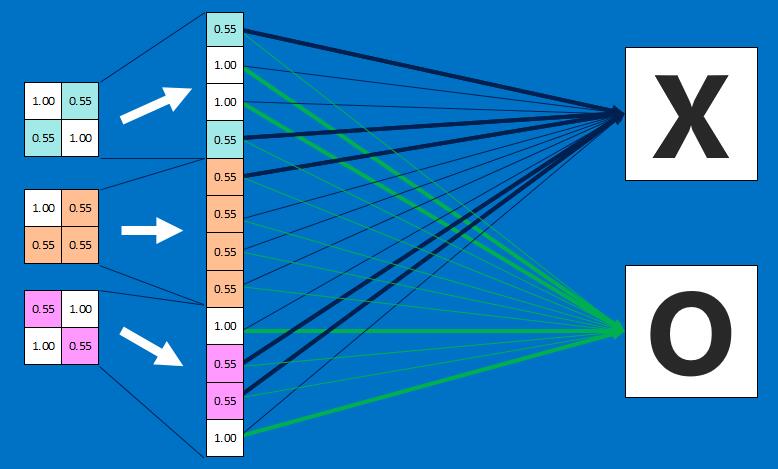
- Fully connected layer