An Overview of Robust Reinforcement Learning
Robust Control Problem
Robust control is an approach to controller design that explicitly deals with uncertainty. Robust control methods are designed to function properly that uncertain parameters or disturbances are found within some set.
Robust methods aim to achieve robust performance and stability in the presence of bounded modelling errors.
In contrast with an adaptive control policy, a robust control policy is static, rather than adapting to measurements of variations, the controller is designed to work assuming that certain variables will be unknown but bounded.
A controller designed for a particular set of parameters is said to be robust if it also works well under a different set of assumptions.
Robust MDP
Robust MDP is an extension of MDP in which the uncertainty of the model is captured by considering transition probabilities to be unknown but bounded in some a priori known uncertainty set.
- Consider a class of models.
- Find the robust optimal policy which is a policy that performs best under the
worst model. - The robust optimal policy satisfies the
robust Bellman equation.
Robust Dynamic Programming
The value of a policy is the minimum expected reward over the set of associated measures, and the goal of the decision maker is to choose a policy with maximum value, we adopt a maximin approach, and refer to this formulation as robust DP.
Motivation
The objective of the robust formulation is to systematically mitigate the sensitivity of the DP optimal policy to ambiguity in the underlying transition probabilities.
Typically, the transition probability of the MDP is estimated from historical data, therefore, subject to statistical errors. In current practice, these errors are ignored and the optimal policy is computed assuming that the estimate is, indeed, the true transition probability. The DP optimal policy is quite sensitve to perturbations in the transition probability and ignoring the estimation errors can lead to serious degradation in performance.
Finite horizon robust DP
The minimum expected value function:
\[V_\pi (s) = \inf_{p \in P^\pi} \mathbb{E}^p \left[ \sum_{t \in T} r_t(s_t, a_t, s_{t+1}) + r_N(s_N) \right], \quad T = \{0,1,2,\cdots,N-1\}.\]The goal of robust DP is to characterize the robust value function:
\[V_*(s) = \sup_{\pi \in \Pi} \left\{ \inf_{p \in P^\pi} \mathbb{E}^p \left[ \sum_{t \in T} r_t(s_t,a_t,s_{t+1}) + r_N(s_N) \right] \right\}, \quad T = \{0,1,2,\cdots,N-1\}.\]The optimal policy \(\pi^*\) if the supremum is achieved.
Robust Bellman function:
Infinite horizon robust DP
The expected reward:
\[V_\pi (s) = \inf_{p \in P^\pi} \mathbb{E}^p \left[ \sum_{t=0}^\infty \gamma^t r(s,a) \right].\]The optimal reward in state \(s\) is given by:
\[V_*(s) = \sup_{\pi \in \Pi} \{ V_\pi(s) \} = \sup_{\pi \in \Pi} \left\{ \inf_{p \in P^\pi} \mathbb{E}^p \left[ \sum_{t=0}^\infty \gamma^t r(s,a) \right] \right\}.\]Robust Bellman function:
Models of uncertainty on transition probability
Likelihood Model
\[\left\{ P \in \mathbb{R}^{n \times n}: P \ge 0, P^T \mathbf{1} = 1, \sum_{i,j} F(i,j) \log P(i,j) \ge \beta \right\},\]where \(F\) is the matrix of empirical frequencies of transition (the observed distribution), \(\beta\) is a given number, which represents the uncertainty level.
Entropy Model
The uncertainty on the \(i\)th row of the transition matrix \(P\) described by a set of the form:
\[p := \left\{ p \vert D(p \Vert q) \le \beta \right\},\]where \(\beta > 0\) is fixed, \(q > 0\) is a given distribution.
Interval Matrix Model
\[p := \left\{ p \big\vert \underline{p} \le p \le \overline{p}, p^T \mathbf{1} = 1 \right\},\]where \(\underline{p}, \overline{p}\) are given componentwise nonnegative \(n\)-vectors, whose elements do not necessarily sum to one.
Robust Model-Free RL
Model misspecification: do not have access to the true environment but only to a reasonably close approximation to it.- Address the problem by extending the framework to
model-free RLsetting, where we do not have access to the model parameters, but can onlysample statesfrom it. - Robust
Q-Learning,SARSA,TD-Learning. - Scale up the robust algorithms to
large MDPsviafunction approximation. - Define an appropriate
Mean Squared Robust Projected Bellman Error (MSRPBE)loss function for stochastic gradient descent algorithms.
Uncertainty Sets
It is easy to have a confidence region \(U_s^a\) (e.g. a ball or an ellipsoid) corresponding to every state-action pair \(s \in S, a \in A\) that quantifies the uncertainty in the environment. Then, the uncertainty region \(P_s^a\) of the probability transition matrix corresponding to \((s,a)\) is defined as
where \(p_s^a\) is the unknown state transition probability vector from the state \(s \in S\) to every other state in \(S\) given action \(a \in A\) during the simulation.
For example, the ellipsoid1 \(U_s^a\) can be defined as
\[U_s^a := \left\{ x \big\vert x^T \Lambda_s^a x \le 1, \sum_{s \in S} x_s = 0, -p_{ss'}^a \le x_{s'} \le 1-p_{ss'}^a, \forall s' \in S \right\},\]where \(\{\Lambda_s^a\}_{s,a}\) is a sequence of positive semidefinite matrices.
For parallelepiped \(U_s^a\),
\[U_s^a := \left\{ x \big\vert \Vert B_s^a x \Vert_1 \le 1, \sum_{s \in S} x_s = 0, -p_{ss'}^a \le x_{s'} \le 1-p_{ss'}^a, \forall s' \in S \right\},\]where \(\{B_s^a\}_{s,a}\) is a sequence of invertible matrices. A constraint \(-p_{ss'}^a \le x_{s'} \le 1-p_{ss'}^a\) is used since we do not have knowledge of \(p_s^a\).
Robust Q-Learning
\[Q^*(s,a) = r(s,a) + \gamma \sigma_{P_s^a}(V^*) = r(s,a) + \gamma \sigma_{U_s^a}(V^*) + \gamma \sum_{s' \in S} p_{ss'}^a \min_{a' \in A} Q^*(s',a'),\]where \(\sigma_P(V) = \sup \{ p^T V \vert p \in P \}\).
Then, the robust Q-iteration is defined as
\[Q_t(s,a) = (1-\lambda)Q_{t-1}(s,a) + \lambda \left( r_t(s,a) + \gamma \sigma_{U_s^a}(V_{t-1}) + \gamma \min_{a' \in A}Q_{t-1}(s',a') \right),\]where the state \(s' \in S\) is sampled with the unknown transition probability \(p_{ss'}^a\) using the simulator.
Robust TD-Learning
TD(0):
\[\delta_t = r(s_t,a_t) + \gamma V_t(s_{t+1}) - V_t(s_t).\]TD(\(\lambda\)) iteration:
\[V_{t+1}(s_k) = V_t(s_k) + \alpha\left( \sum_{t=k}^\infty (\lambda\gamma)^{t-k} \delta_t \right).\]Define the robust TD-error as
\[\tilde{\delta}_t = \delta_t + \gamma \sigma_{U_{s_t}^{\pi(s_t)}}(V_t).\]Robust RL for Continuous Control
Robust RL aims to derive an optimal behavior that accounts for model uncertainty in dynamical systems.
Motivation
The current crop of RL agents are typically trained in a single environment. Therefore, an issue that is faced by many of these agents is the sensitivity of the agent's policy to environment perturbations. Perturbing the dynamics of the environment during test time, which may include executing the policy in a real-world setting, can have a significant negative impact on the performance of the agent.
Environment perturbations: lighting, weather conditions, sensor noise, actuator noise, action delays, etc.
An agent is trained in one environment and performs poorly in a different, perturbed version of the environment is considered as model misspecification. Robust RL focuses on robustness to model misspecification in the transition dynamics.
A robust policy optimizes for the worst-case expected return objective.
Maximum A-Posteriori Policy Optimization (MPO)
Policy evaluation
Input a policy \(\pi_k\) and evaluates an action-value function \(Q_\theta^{\pi_k}(s,a)\) by minimizing the squared TD-error:
\[\min_\theta \left( r(s,a) + \gamma Q_{\hat{\theta}}^{\pi_k}(s',a') - Q_\theta^{\pi_k}(s,a) \right)^2.\]Robust policy evaluation
Optimize the worst-case squared TD-error:
\[\min_\theta \left( r(s,a) + \gamma \inf_{p \in P(s,a)} \left[ Q_{\hat{\theta}}^{\pi_k}(s',a') \right] - Q_\theta^{\pi_k}(s,a) \right)^2.\]Robust Entropy-Regularized policy evaluation
Entropy regularization encourages exploration and helps prevent early convergence to sub-optimal policies.
Robust entropy-regularized Bellman equation:
\[V(s) = \mathbb{E}_{a \sim \pi(\cdot \vert s)} \left[ r(s,a) - \tau \log \frac{\pi(\cdot \vert s)}{\bar{\pi}(\cdot \vert s)} + \gamma \inf_{p \in P} \mathbb{E}_{s' \sim p(\cdot \vert s,a)}[V(s')] \right].\]Robust Entropy-regularized squared TD-error:
\[\min_\theta \left( r(s,a) + \gamma \inf_{p \in P(s,a)} \left[ \widetilde{Q}_{\hat{\theta}}^{\pi_k}(s',a';\bar{\pi}) - \tau KL(\pi_k(\cdot \vert s') \Vert \bar{\pi}(\cdot \vert s')) \right] - \widetilde{Q}_\theta^{\pi_k}(s,a;\bar{\pi}) \right)^2.\]Soft-Robust Reinforcement Learning
Motivation
Previous studies have shown the robust RL by considering the worest case scenario, robust policies can be overly conservative. The soft-robust framework is an attempt to overcome this issue.
Soft-Robust Actor-Critic Policy Gradient
It learns an optimal policy w.r.t. a distribution over an uncertainty set and stays robust to model uncertainty but avoids the conservativeness of robust strategies (aggressive and robust).
The uncertainty transition probability distribution over \(P\) is denoted by \(w\) and is structured as a cartesian product \(\otimes_{s \in S} w_s\) (Eg. \(A = \{a,b\}\), \(B = \{0,1,2\}\), the cartesian product of the two sets is \(\{(a,0),(a,1),(a,2),(b,0),(b,1),(b,2)\}\)). Intuitively, \(w\) can be thought as the way the adversary distributes over different transition models.
The soft-robust objective function:
\[\bar{J}(\pi) = \mathbb{E}_{p \sim w}[J_p(\pi)].\]Define the average transition model as:
\[\bar{p} := \mathbb{E}_{p \sim w}[p].\]The stationary distribution of the average transition model is:
\[\bar{d}^\pi(s) = \mathbb{E}_{p \sim w}[d_p^\pi (s)], \quad s \in S.\]Then, the objective function is:
The goal is to learn a policy that maximizes the soft-robust objective function \(\bar{J}\).
Soft-robust policy gradient:
where
\[\bar{Q}^\pi (s,a) = \mathbb{E}_{p \sim w}[Q_p^\pi(s,a)].\]To reduce the variance, one direct method is to subtract a baseline \(\bar{V}^\pi(s)\):
where
\[\bar{A}^\pi (s,a) := \bar{Q}^\pi(s,a) - \bar{V}^\pi(s).\]Algorithm of Soft-Robust AC
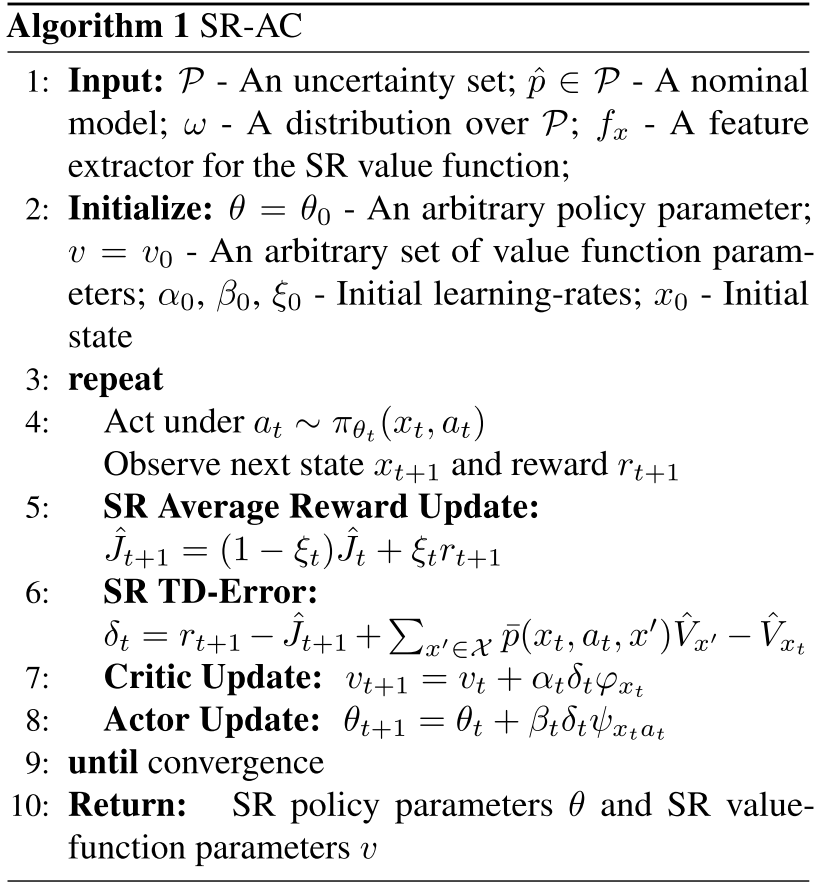
- SR-AC Algorithm Pseudocode
Experiments
- Single-step MDP
- discrete state and action space
- 5 different probabilities of success using a uniform distribution over \([0, 1]\)
SR-AC
- Cart-Pole
- continuous state space \(\langle x, \dot{x}, \theta, \dot{\theta} \rangle\) and discrete action space (left or right)
- 5 different lengths from a normal distribution
SR-DQN
- Pendulum
- continuous state \(\langle \theta, \dot{\theta} \rangle\) and action \([-a, a]\) space
- 10 different masses of pendulum around a nominal mass of 2
SR-DDPG
For each experiment, generate an uncertainty set \(P\) before training. Each corresponding model thus generate a different transition function. Then, sample the average model by fixing \(w\) as a realization of a Dirichlet distribution. A soft-robust update for the actor is applied by taking the optimal action according to this average transition function.
SR-AC
Run a regular AC algorithm to derive an aggressive policy.
Learn a robust policy by using a robust formulation of TD-error to replace the nominal TD-error.
SR-DQN
Robust TD-error:
Soft-Robust TD-error:
SR-DDPG
Robust TD-error:
Soft-Robust TD-error: