Deep Drone Acrobatics

Motivation

Acrobatic flight requires high thrust and extreme angular accelerations that push the platform to its physical limits.

Human drone pilots require many years of practice to safely master maneuvers such as power loops and barrel rolls.

Existing autonomous systems that perform agile maneuvers require external sensing and external computation.

Acrobatic maneuvers represent a challenge for the actuators, sensors, and all physical components of a quadrotor.

Limiting Factor

• The major limiting factor to enable agile flight is reliable state estimation.
• The harsh requirements of fast and precise control at high speeds make it difficult to tune controllers on the real platform.

Limits of vision-based state estimation systems:

• provide significantly reduced accuracy.
• completely fail at high accelerations due to effects such as motion blur, large displacements, and the difficulty of robustly tracking features over long time frames.

Two Research Lines

• Control problem: state estimation from external sensors (Vicon or OptiTrack).
• Address the control and perception aspects in an integrated way
  • Perception-guided trajectory optimization.
  • Training end-to-end visuomotor agents.

Contributions

• Propose to learn an end-to-end sensorimotor policy that enables an autonomous quadrotor to fly extreme acrobatic maneuvers.
  • Input: conbine information from different sensors.
    • Employ abstraction of sensory input to reduce the problem's sample complexity and enable zero-shot sim-to-real transfer.
    • Design asynchronous network to cope with different output frequencies of the onboard sensors.
  • Output: thrust and body rates.
• Simulation-to-reality transfer strategy: Train acrobatic controllers in simulation and deploy them with no fine-tuning (zero-shot transfer) on physical quadrotors.
• Advantages of simulation:
  • maneuvers can be simply specified by reference trajectories in simulation, do not require expensive demonstrations by a human pilot.
  • Training is safe.
  • The approach can scale to a large number of diverse maneuvers.
• Use only onboard sensing (vision-based, IMU) and computation.
• Acrobatics
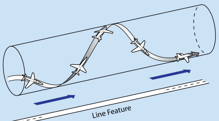
  • Barrel Roll
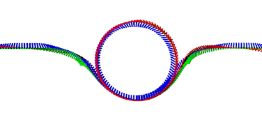
  • Power Loop
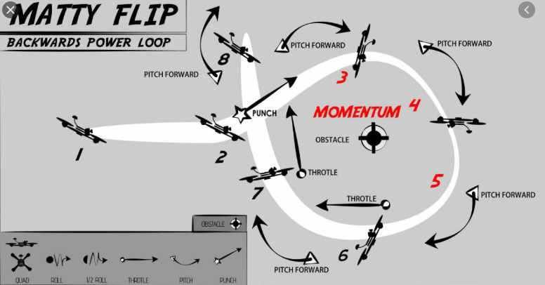
  • Matty Flip

Method

• Train the policy entirely in simulation by leveraging demonstrations from an optimal controller that has access to privileged information.
  • need a history of onboard sensor measurements.
  • need a user-defined reference trajectory.
• Use appropriate abstractions of the visual input to enable transfer to a real quadrotor. The resulting policy can be directly deployed in the physical world without any fine-tuning on real data.
• It does not require a human expert to provide demonstrations.
• During the acrobatic flight, the quadrotor incurs accelerations of up to 3g.
• Video: https://www.youtube.com/watch?v=2N_wKXQ6MXA&feature=youtu.be
• Code: https://github.com/uzh-rpg/deep_drone_acrobatics

Observation

An observation \(o[k] \in \mathbb{O}\) at time \(k \in [0,\cdots,T]\) consists of:

• a camera image \(I[k]\): feature points extracted via classic computer vision.
• an IMU \(\phi[k]\).

Since the camera and IMU typically operate at different fraquencies, the visual and inertial observations are updated at different rates.

Action

The controller’s output is an action \(u[k] = [c,w^T]^T \in \mathbb{U}\) consists of:

• continuous mass-normalized collective thrust \(c\).
• body rates \(w = [w_x,w_y,w_z]^T\).

Algorithm

Privileged learning: the policy is trained on demonstrations that are provided by a privileged expert, which is an optimal controller (based on a classic optimization-based planning and control pipline that tracks a reference trajectory from the ground-truth state using MPC) that has access to privileged information that is not available to the sensorimotor student, such as the full ground-truth state of the platform \(s[k] \in \mathbb{S}\).

Collect training demonstrations from the privileged expert in simulation.

Training in simulation enables synthesis and use of unlimited training data for any desired trajectory.

The sensorimotor policy does not directly access raw sensor input such as color images, but the abstraction of the image, in form of feature points extracted via classic computer vision.

The trained sensorimotor policy does not rely on any privileged information and can be deployed directly on the physical platform.

Problem definition

Define the task of flying acrobatic maneuvers with a quadrotor as a discrete-time, continuous-valued optimization problem.

Objective

To find an end-to-end control policy:

which is defined by a neural network to minimize the following finite-horizon objective:

where

• \(C\) is a quadratic cost.
• \(\tau_r[k]\) is a reference trajectory.
• \(s[k]\) is the quadrotor state, \(s[k]=[p,q,v,w]\), the agent does not directly observe the state.
• \(\rho(\pi)\) is the distribution of possible trajectories \(\{ (s[0],o[0],u[0]), \cdots, (s[T],o[T],u[T]) \}\) induced by the policy \(\pi\).

Formulate the cost \(C\) as

where \(x[k]=\tau_r[k]-s[k]\) denotes the difference between the state of the quadrotor and the corresponding reference at time \(k\), and \(L\) is a positive-semidefinite cost matrix.

Reference Trajectories

To ensure that the reference trajectory is dynamically feasible, it has to satisfy constraints:

• physical limits.
• underactuated nature of the quadrotor platform.

Dynamics of the quadrotor can be modelled as:

where

• \(p_{WB}, v_{WB}, q_{WB}\) denote the position, linear velocity, and orientation of the body frame w.r.t. the world frame.
• \(g_W\) is the gravity vector in the world frame.
• \(c_B = (0,0,c)^T\) denotes the mass-normalized thrust vector.
• \(q_{WB} = (q_\omega,q_x,q_y,q_z)^T\) is the quaternion.
• \(\Lambda(\omega_B)\) is a skew-symmetric matrix of the the vector \((0,\omega_B^T)^T = (0,\omega_x,\omega_y,\omega_z)^T\).
• \(J = diag(J_{xx},J_{yy},J_{zz})\) denotes the quadrotor inertia matrix.
• \(\eta \in \mathbb{R}^3\) are the torques acting on the body due to the motor thrusts.

Plan the reference trajectories in the space of flat outputs¹:

where \(x,y,z\) denote the position of the quadrotor, and \(\psi\) is the yaw angle. It can be shown that any smooth trajectory in the space of flat ouputs can be tracked by the underactuated platform.

Composition of a reference trajectory:

• enter trajectory
• core part trajectory: a circular motion primitive with constant tangential velocity \(v_l\). To ensure a well-defined reference trajectory through the whole circular maneuver, constrain the norm of the tangential velocity \(v_l\) to be larger by a margin \(\epsilon\) than the critical tangential velocity that would lead to free fall at the top of the maneuver, \(\Vert v_l \Vert > \epsilon \sqrt{rg}\), where \(r\) is the radius of the loop, \(g = 9.81ms^{-2}\), and \(\epsilon=1.1\).
• exit trajectory

The enter, transition between, and exit of the maneuver can be obtained using constrained polynomial trajectories.

A polynomial trajectory is described by four polynomial functions specifying the independent evolution of the components of \(\sigma\) over time:

• \(P_i=7, i=\{1,2,3\}\) for the position components.
• \(P_i=2, i=4\) for the yaw angle component.

Constrain the polynomial trajectory by:

• minimize the execution time \(t_m\) of the polynomial trajectory.
• constrain the maximum speed, thrust, body rates through the maneuver.

Then, all the trajectories are concatenated to the full reference trajectory, and then converted back to the full state space representation \(\tau_r(t)\) using differential flatness.

Differential flatness: 平坦系统具有平坦输出，可以用平坦输出以及其有限微分的组合来显式表示所有的状态和输入。

How can we convert the flat outputs to the full state space?

• position \((x,y,z)\)
• line velocity \((\dot{x}, \dot{y}, \dot{z})\)
• rotation matrix \(^WR_B\)
• angular velocity \(\omega_{BW}\)
• angular acceleration \(\alpha_{BW}\)
• control signals \((u_1,u_x,u_y,u_z)\)

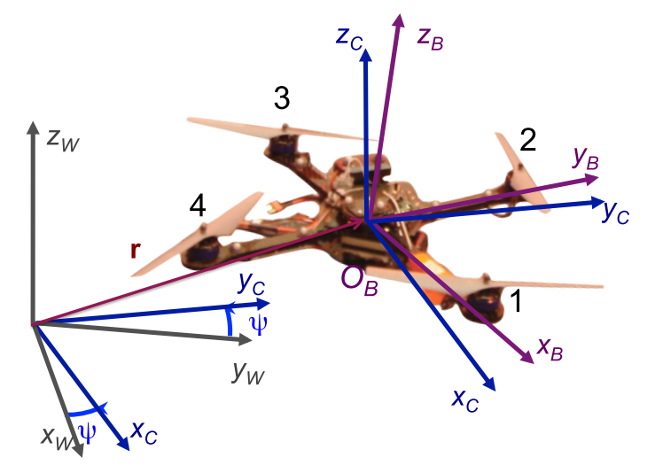
The rotation matrix from \(B\) to \(W\) is given by:

where \(^WR_C\) represents the yaw rotation to the intermediate frame \(C\), and \(^CR_B\) represents the effect of roll and pitch.

Angular velocity of frame \(B\) in \(W\):

The states and control inputs of the quadrotor can be written as algebraic functions of four carefully selected flat outputs and their derivatives.

Define a trajectory, \(\sigma(t)\), as a smooth curve in the space of flat outputs:

Define the body frame \(z\) axis of the quadrotor:

Given the yaw angle \(\sigma_4 = \psi\),

Then,

Thus, we can uniquely determine the rotation matrix:

Newton’s equation of the acceleration is:

Take the first derivative of the above equation:

Projecting the expression along \(\mathbf{z}_B\), using that \(\dot{u}_1 = \mathbf{z}_B \cdot m \dot{a}\), then define the vector \(\mathbf{h_w}\) as

where \(\mathbf{h_w}\) is the projection of \(\frac{m}{u_1}\dot{a}\) onto the \(\mathbf{x}_B-\mathbf{y}_B\) plane.

Then,

The component \(y\) is found by simply writing:

where that \(\omega_{BC}\) has no \(\mathbf{z}_B\) component, then:

Thus, we can obtain the angular velocity \(\omega_{BW}\).

For the components of angular acceleration \(\alpha_{BW}\) along \(\mathbf{x}_B\) and \(\mathbf{y}_B\) are found by computing the second of derivative of the Newton’s equation, then following the same procedure as above.

To find the \(\mathbf{z}_B\) component of the angular acceleration, use

Then

For the control inputs component, the thrust \(u_1\) from the quadrotor propellers can be obtained by

For the control signal of torques \((u_x,u_y,u_z)\), we can obtain from Euler function.

Privileged Expert

Privileged expert policy \(\pi^*\) consists of an MPC and generates collective thrust and body rates via an optimization-based scheme.

The MPC repeatedly optimizes the open-loop control problem over a receding horizon of \(N\) time steps and applies the first control command from the optimized sequence.

The MPC solves the following optimization problem to obtain the action:

where

• \(r(x,u)\) are equality constraints imposed by the system dynamics.
• \(h(x,u)\) are optional bounds on inputs and states.
• \(L,R\) are positive-semidefinite cost matrices.

Policy Learning

Sensorimotor policy:

• training by imitating demonstrations provided by the privileged expert.
• does not access any privileged information.
• directly deployed in the physical world.

Define an upper bound between the expert and the student performance as

where

• \(W(\pi,\pi^*)\) is the Wasserstein metric.
• \(C_{\pi^*}\) is a constant depending on the smoothness of expert actions.

The discrepany can be minimized by an iterative supervised learning algorithm DAGGER².

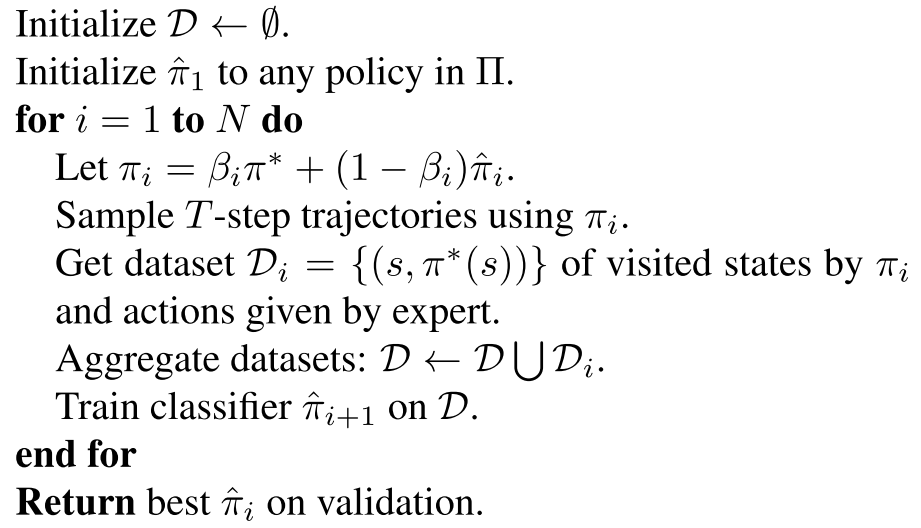
Algorithm of Dataset Aggregation (DAGGER)

Updating the student policy based on supervised learning problem:

where

• \(u^*(s[k])\) is the expert action.
• \(o[k]\) is the observation vector in the state \(s[k]\).

Running the process for \(O(N)\) iterations yields a policy \(\pi\) with performance:

Network Architecture

Define the observation models describe how an onboard sensor measurement \(z\) senses a state \(s\):

• \(M(z \vert s): \mathbb{S} \to \mathbb{O}\) denotes the model in real world.
• \(L(z \vert s): \mathbb{S} \to \mathbb{O}\) denotes the model in simulation.

Define the policies:

• \(\pi_r = \mathbb{E}_{o_r \sim M(s)}[\pi(o_r[k])]\) in real world.
• \(\pi_s = \mathbb{E}_{o_s \sim L(s)}[\pi(o_s[k])]\) in simulation.

The simulation-to-reality gap is upper bounded by:

where \(K\) denotes the Lipschitz constant.

The effect of abstraction of the input observations:

where \(f\) is a mapping of the abstraction of camera frames which is provided by a visual-inertial odometry (VIO).

Thus, from the above equation, we know that a policy acts on an abstract representation of the observations \(\pi_f: f(\mathbb{O}) \to \mathbb{U}\) has lower simulation-to-reality gap that a policy \(\pi_o: \mathbb{O} \to \mathbb{U}\) that acts on raw observations.

Challenges:

• keep track its state.
• not require retraining for each scene.
• process sensor readings that are provided at different frequencies.

Inputs of the network:

• visual: 15Hz, 5D vector, keypoint position, displacement w.r.t. previous keyframe, number of keyframes that the feature has been tracked (a measure of keypoint quality), random sample 40 keypoints per keyframe, a history of feature track keypoints (Harris corners) in the image plane extracted by VINS-Mono.
• IMU: 100Hz, velocity, orientation, angular rate, preprocess the IMU signal by applying bias subtraction and gravity alignment.
• reference trajectory: 50Hz, velocity, orientation, angular rate.

Experiment

Platform

• Simulation
  • Gazebo
  • RotorS-ETH
  • AscTec Hummingbird: equipped with a forword-facing fisheye camera
  • World: space with a side length of 70 meters
• Experiment
  • Quadrotor: 1.15kg, has a thrust-to-weight ratio 4:1
  • Jetson TX2: neural network inference
  • Intel RealSense T265 camera: images, IMU

Learning Process

• off-policy
  • execute the trained policy, collect rollouts, add them to a dataset.
  • after 30 new rollouts are added, train for 40 epochs on the entire dataset.
  • repeat 5 times of the collect-rollouts-train procedure.
  • there are 150 rollouts in the dataset.
  • use Adam optimizer with a learning rate \(3e-4\).
  • perform a random action with a probability \(p=30\%\) at every stage of the training to increase the coverage of the state space.

Evaluation

Solve the following questions:

• Sensorimotor policy VS State estimation and control?
• What is the role of input abstraction in facilitating transfer from simulation to reality?

Learning policies for the following acrobatic maneuvers:

• Power Loop: Accelerate over a distance of 4m to a speed of 4.5m/s, enter a loop with a radius of 1.5m.
• Barrel Roll: Accelerate over a distance of 3m to a speed of 4.5m/s, enter a loop with a radius of 1.5m.
• Matty Flip: Accelerate over a distance of 4m to a speed of 4.5m/s while yawing 180deg, enter a loop with a radius of 1.5m.
• Combo: start with a triple Barrel Roll, followed by a double Power Loop, and ends with a Matty Flip.

Comparison method:

• a strong baseline by combining VIO and MPC
  • receive the same inputs: IMU, Image, Reference trajectory.

Metrics:

• Simulation:
  • the average root mean square error in meters of reference position w.r.t. the true position of the platform during the execution of the maneuver.
• Real world:
  • the average success rate as not crashing the platform into any obstacles during the maneuver.
  • a maneuver successful if the pilot did not have to intervene during the execution and the maneuver was executed correctly.

Code

custom rotors interface

• Subscribe
  • control command: control_command = *msg rate_cmd: \((\omega_x,\omega_y,\omega_z,C)\)
  • arm: interface_armed = true
  • autopilot: autopilot_feedback = *msg
  • odometry: odometry = *msg body_rate_estimate: \((\hat{\omega}_x,\hat{\omega}_y,\hat{\omega}_z)\)
  • motor speed: \((\omega_0^t, \omega_1^t, \omega_2^t, \omega_3^t)\)
• Public
  • motor speed: \((\omega_0^{t+1}, \omega_1^{t+1}, \omega_2^{t+1}, \omega_3^{t+1})\)

Humingbird platform:

    0 cw               x
    |                  |
1---+---3 ccw    y <---+
    |
    2 cw

Use the subscribed motor speed \((\omega_0^t, \omega_1^t, \omega_2^t, \omega_3^t)\) to estimate the body torques and thrust at time step \(t\):

Control error \(e\):

where \(\tau^t = [\tau_x^t,\tau_y^t,\tau_z^t]^T\), \(\omega = [\omega_x,\omega_y,\omega_z]^T\).

LQR controller:

Let the state space as \(s = [\omega\quad \tau]^T\).

Linearizing the state equation as:

Then, design the LQR control law as:

Minimize the following cost function:

Then,

Corresponding to a PD controller of the body rates:

Where

• \(\hat{\omega}\times (J\hat{\omega})\) is the feedback linearization compensating for the coupling terms in the body rates dynamics.
• \(J\dot{\omega}\) is a feed-forward term on the desired angular accelerations.

Mixer:

Public the motor speed \((\omega_0^{t+1}, \omega_1^{t+1}, \omega_2^{t+1}, \omega_3^{t+1})\) at time step \(t+1\).

References