Trajectory Generation for UAV Control
Path Planning VS Trajectory Planning VS Motion Planning
| Index | Path Planning | Trajectory Planning | Motion Planning |
|---|---|---|---|
| Dimension | Space | Space + Time | Space + Time |
| Constraints | Kinematics | Kinematics + Dynamics (balance, joint limits, torque bounds, velocity/acceleration/jerk limits) | Kinematics + Dynamics + Environments (collision avoidance) |
| Process | Planning + Waypoints | Planning + Generation | Planning + Generation + Controller |
| Output | Path | Path + Speed (Acceleration, Jerk) | Discrete Motions / Commands |
Challenges
- How to define the optimal trajectory?
- cost function
- energy consumption
- objective function
- travel length
- cost function
- Optimization methods:
- discrete method
- search-based
- sampling-based
- continuous method
- optimization-based
- discrete method
- Constraints:
- dynamics limits
- kinematic limits
- obstacle avoidance
- Trajectory optimization:
- smoothness
- consider uncertainty
Trajectory Planning
- Known as a movement from
starting pointtoending pointby satisfying theconstraintsalong the path. - It is an essential part of robot
motion planning. - Planning high-speed trajectories for UAV in
unknown environmentsrequires:- fast algorithms able to solve the
trajectory generationproblem inreal-timein order to be able toreact quickly to the changing knowledge of the worldand that guarantee safety at all times. - Dynamical feasible:
- Satisfy the physical limits.
- The underactuated nature of the quadrotor.
- fast algorithms able to solve the
Trajectory Generation
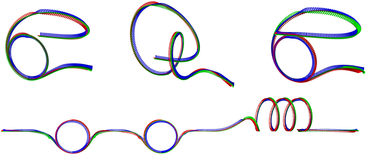
Top: Power Loop, Barrel Roll, Matty Flip, Bottom: Combo.
A. Loquercio, E. Kaufmann, and D. Scaramuzza, “Deep Drone Acrobatics,” RSS Robot. Sci. Syst., 2020.
Instead of directly planning in the full state space, generating the trajectory in the space of flat outputs:
It can be shown that any smooth trajectory in the space of flat outputs can be tracked by the underactuated platform.
Polynomial trajectory
Motivation
Consider the problem of navigating through \(m\) keyframes (waypoints) at specified times.
In between each keyframe there is a safe corridor that the quadrotor must stay within.
We can use straight lines to interpolate between keyframes. However, the trajectory is inefficient because it has infinite curvature at the keyframes, which requires the quadrotor to come to a stop at each keyframe.
Polynomial functions can fit out an optimal trajectory that smoothly transitions through the keyframes at the given times while staying within safe corridors.
Constraints of the trajectory
Enforce some limits when designing a trajectory:
- Maximum Speed: \(v_{max}\).
- Maximum Collective thrust: \(F_{T_{max}}\).
- Maximum norm of the roll and pitch rates: \(\omega_{max}\).
The limits of the trajectory need to be computed from a desired state sampled from the given trajectory:
Speed
\[v = \lVert v_{des} \rVert.\]Collective thrust
\[F_T = \lVert a_{des} - g \rVert.\]The norm of the roll and pitch rates
In world frame,
\[F = a_{des} - g = R\cdot \mathbf{F_T}.\]Then,
\[\bar{F} = \frac{F}{\lVert F \rVert} = R\cdot\begin{bmatrix} 0 \\ 0 \\ 1 \end{bmatrix}.\]Take the derivative:
\[\dot{\bar{F}} = \dot{R} \cdot\begin{bmatrix} 0 \\ 0 \\ 1 \end{bmatrix} = R \hat{\omega}\cdot\begin{bmatrix} 0 \\ 0 \\ 1 \end{bmatrix}.\]Then,
\[\hat{\omega}\cdot\begin{bmatrix} 0 \\ 0 \\ 1 \end{bmatrix} = R^T \dot{\bar{F}},\] \[\begin{bmatrix} \omega_y \\ -\omega_x \\ 0 \end{bmatrix} = R^T\dot{\bar{F}}.\]Where
\[\dot{\bar{F}} = \frac{d}{dt}\left( \frac{F}{\lVert F \rVert} \right) = \frac{\dot{F}\lVert F \rVert - F\frac{F^T \dot{F}}{\lVert F \rVert}}{\lVert F \rVert^2} = \frac{\dot{F}}{\lVert F\rVert} - \frac{FF^T\dot{F}}{\lVert F\rVert^3} = \frac{j}{\lVert F\rVert} - \frac{FF^Tj}{\lVert F\rVert^3}.\]Thus,
\[\begin{aligned} \begin{bmatrix} \omega_y \\ -\omega_x \\ 0 \end{bmatrix} & = R^T \left( \frac{j}{\lVert F\rVert} - \frac{FF^Tj}{\lVert F\rVert^3} \right) \\ & = R^T \frac{j}{F_T} - R^T\frac{R\mathbf{F_T} \mathbf{F_T}^T R^T j}{F_T^3} \\ & = R^T \frac{j}{F_T} - \frac{\mathbf{F_T} \mathbf{F_T}^T R^T j}{F_T^3}. \end{aligned}\]Where
\[\mathbf{F_T} \mathbf{F_T}^T = \begin{bmatrix} 0 & 0 & 0 \\ 0 & 0 & 0 \\ 0 & 0 & F_T^2 \end{bmatrix}.\]Then,
\[\begin{bmatrix} \omega_y \\ -\omega_x \\ 0 \end{bmatrix} = \begin{bmatrix} x_B^T\cdot \frac{j}{F_T} \\ y_B^T\cdot \frac{j}{F_T} \\ z_B^T\cdot \frac{j}{F_T} \end{bmatrix} - \begin{bmatrix} 0 \\ 0 \\ z_B^T \cdot \frac{j}{F_T} \end{bmatrix}.\] \[\lVert R^T \cdot \frac{j}{F_T}\rVert = \lVert\frac{j}{F_T}\rVert.\] \[z_B = \frac{a_{des} - g}{\lVert a_{des} - g\rVert}.\]Therefore, the norm of the roll and pitch body rates:
\[\lVert \omega_{x,y}\rVert = \left\Vert \begin{bmatrix} \omega_y \\ -\omega_x \\ 0 \end{bmatrix} \right\Vert = \sqrt{\left\Vert \frac{j}{F_T} \right\Vert^2 - \left( z_B^T\frac{j}{F_T} \right)^2}.\]Polynomial Coefficients
The goal of polynomial trajectory generation is to obtain the polynomial coefficients which satisfy some constraints.
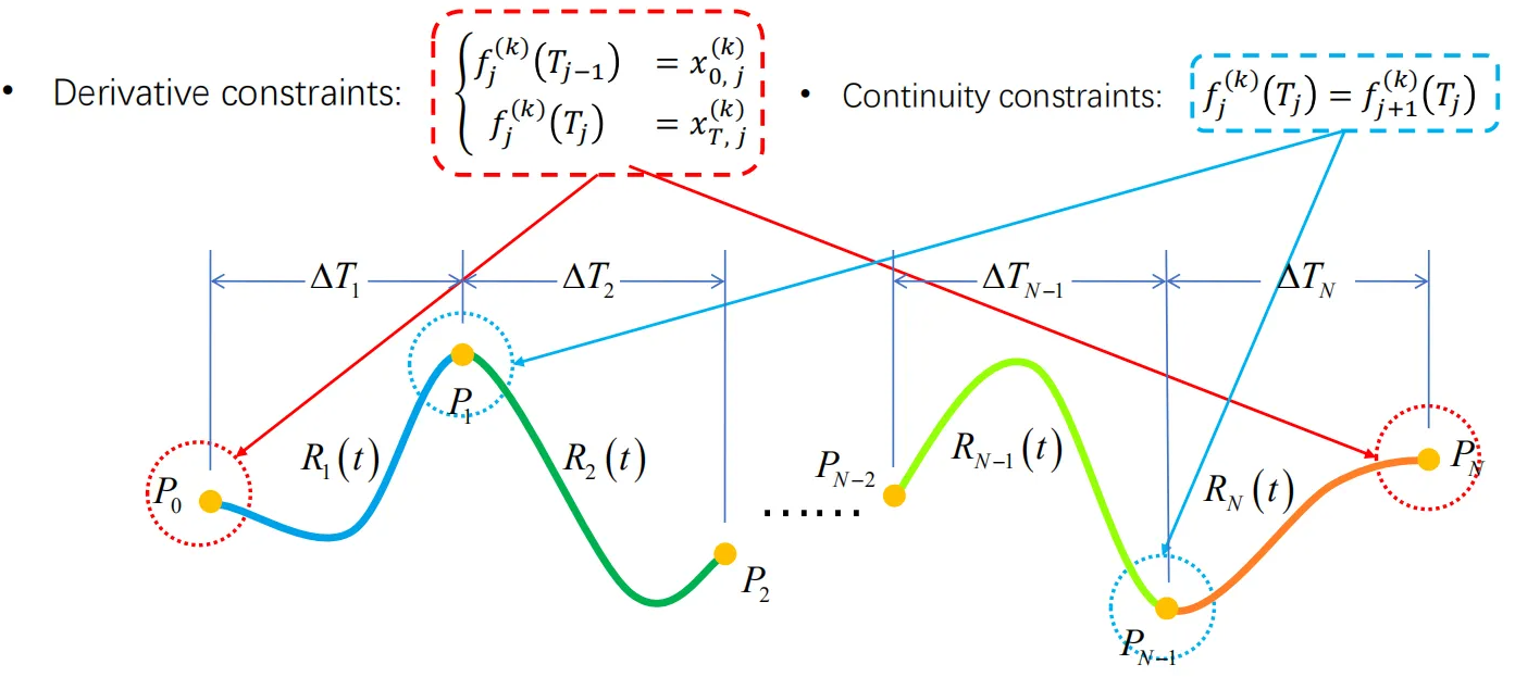
A piecewise-smooth trajectory can be generated by piecewise polynomial functions of order \(n\) over \(m\) keyframes time intervals (\(m\) segments, add the start state):
Write as matrix form:
\[\sigma(t) = \begin{cases} \sigma_1\cdot [1,t,t^2,\cdots,t^n] & t_0 \le t < t_1 \\ \sigma_2\cdot [1,t,t^2,\cdots,t^n] & t_1 \le t < t_2 \\ \vdots \\ \sigma_m\cdot [1,t,t^2,\cdots,t^n] & t_{m-1} \le t \le t_{m}. \end{cases}\]Where \(\sigma^j, j = \{1,\cdots,m\}\) is the polynomial coefficient matrix (\(4\times (n+1)\)) of the \(j\)th piecewise trajectory.
For each piecewise trajectory polynomial:
\[\sigma(t) = \sigma_{4\times (n+1)} \cdot [1,t,t^2,\cdots,t^n].\]Then, for anytime \(t\), the position \(p_t\), velocity \(v_t\), acceleration \(a_t\), jerk \(j_t\), and snap of the trajectory can be calculated by:
\[\begin{aligned} p_t & = \sigma_{3\times (n+1)} \cdot [1,t,t^2,t^3,t^4,t^5,\cdots,t^n], \\ v_t & = \sigma_{3\times (n+1)} \cdot [0,1,2t,3t^2,4t^3,5t^4,\cdots,nt^{n-1}], \\ a_t & = \sigma_{3\times (n+1)} \cdot [0,0,2,6t,12t^2,20t^3,\cdots,n(n-1)t^{n-2}], \\ j_t & = \sigma_{3\times (n+1)} \cdot [0,0,0,6,24t,60t^2,\cdots,\frac{n!}{(n-3)!}t^{n-3}], \\ snap_t & = \sigma_{3\times (n+1)} \cdot [0,0,0,0,24,120t,\cdots,\frac{n!}{(n-4)!}t^{n-4}]. \end{aligned}\]Minimum Snap Trajectory
Why minimize snap?1
- Minimizing the control effort, do this indirectly by minimizing snap.
- The
thrustsis related to the second derivatives of the curve. - The
torquesof control inputs appear as functions of the fourth derivatives of the positions. - Minimizing snap will give us the curve that requires the least reorientation of the quadrotor along it, and will guarantee smoothness.
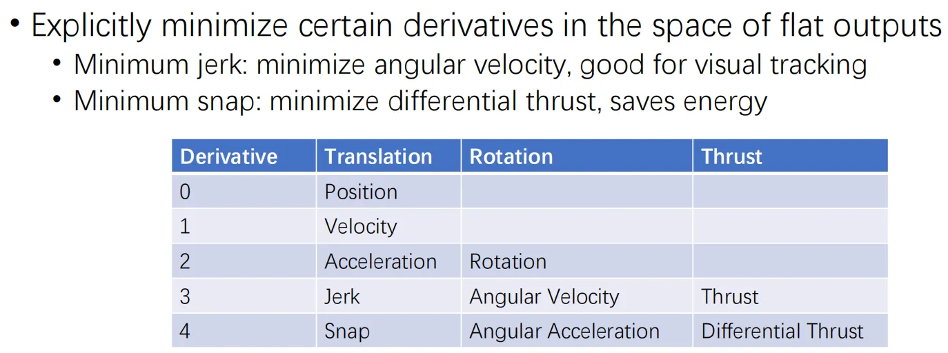
The optimization program to solve this problem:
- Minimize the integral of the \(k_p\)th derivative of position squared.
- \(k_p = 4\), minimize the integral of the square of the norm of the
snap.
- \(k_p = 4\), minimize the integral of the square of the norm of the
- Minimize the integral of the \(k_\psi\)th derivative of yaw angle squared.
- \(k_\psi = 2\).
Cost function:
\[\min \int_{t_0}^{t_{m}} \mu_p \left\Vert \frac{d^{k_p}p_t}{dt^{k_p}}\right\Vert^2 + \mu_\psi \left\Vert \frac{d^{k_\psi}\psi_t}{dt^{k_\psi}}\right\Vert^2 dt,\] \[s.t. \begin{cases} \sigma(t_i) = \sigma_i & i = 0,\cdots, m \\ \frac{d^k p_t}{dt^k}\vert_{t = t_j} = 0 \text{ or free} & j = 0,m; k = 1,\cdots,k_p \\ \frac{d^k \psi_t}{dt^k}\vert_{t = t_j} = 0 \text{ or free} & j = 0,m; k = 1,\cdots,k_\psi. \end{cases}\]where
- \(\mu_p,\mu_\psi\) are constants that make the integrand nondimensional.
Formulate the problem as a quadratic program (QP) by:
For minimize snap:
Where \(r,c\) are the index of row and column.
Constraints:
- Equality constraints.
- At \(t_0\):
- \(\sigma_{3\times (n+1)} \cdot [1,t_0,t_0^2,t_0^3,t_0^4,t_0^5,\cdots,t_0^n] = p_0\).
- Also, \(v_0,a_0,j_0\).
- Similar, \(p_k,v_k,a_k\).
- At \(t_0\):
- Inequality constraints.
- Used in corridor environment.
- \(p_k \le p_{max}\).
- Similar, \(v_k,a_k\).
Then, using QP solver (Lagrangian method) to calculate the polynomial coefficients.
Add corridor constraints
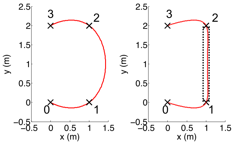
Define the unit vector along the segment from \(\mathbf{p}_j\) to \(\mathbf{p}_{j+1}\) as:
\[\mathbf{N}_j = \frac{\mathbf{p}_{j+1} - \mathbf{p}_j}{\Vert \mathbf{p}_{j+1} - \mathbf{p}_j \Vert}.\]The perpendicular distance from segment \(j\) is defined as:
\[\mathbf{d}_j(t) = (\mathbf{p}(t) - \mathbf{p}_j) - ((\mathbf{p}(t) - \mathbf{p}_j)\mathbf{N}_j)\mathbf{N}_j.\]A corridor width on the infinity norm is defined for each corridor:
\[\Vert \mathbf{d}_j(t)\Vert_\infty \le \delta_j, \quad t_j \le t \le t_{j+1}.\]The constraint can be incorporated into the QP by introducing \(n\) intermediate points as:
\[\left\vert \mathbf{x}_W\cdot \mathbf{d}_j\left( t_j + \frac{i}{1+n}(t_{j+1} - t_j) \right)\right\vert \le \delta_j, \quad i = 1, \cdots, n.\]Equivalently for \(\mathbf{y}_W, \mathbf{z}_W\).
Optimal segment times
The arrival times at different keyframes is important and may be specified.
Try to find a better solution by allowing more time for some segments while taking the same amount of time away from the others.
Describe a method for finding the optimal relative segment times for a given set of keyframes.
For \(T_j = t_j - t_{j-1}\), solve the minimization problem:
\[\min f(\mathbf{T})\] \[s.t.\begin{cases} \sum_{j=1}^m T_j = t_m \\ T_j \ge 0. \end{cases}\]Where \(\mathbf{T} = [T_1,T_2,\cdots,T_m]\).
Solving the optimization problem via a constrained gradient descent method.
Computing the directional derivative by:
\[\nabla_{g_j}f = \frac{f(\mathbf{T}+h\mathbf{g}_j) - f(\mathbf{T})}{h},\]where
- \(h\) is some small number.
- \(\mathbf{g}_j\) is constructed that the \(j\)th element has a value of \(1\), and all other elements have the value \(\frac{-1}{m-2}\).
- \(\sum\mathbf{g}_j = 0\).