An Overview of A* Algorithms

路径搜索算法

Path Planning: 依据某个或某些优化准则（路径最短、时间最短等），在工作空间中找到一条从起始状态到目标状态且能避开障碍物的最优路径。

静态环境路径搜索：
- A*
动态环境路径搜索：移动障碍物。
- D*, 1994(Stentz)¹:
  - Dynamic A*.
  - 动态启发式路径搜索。
  - 不需要预先探明地图。
  - 美国火星探测器寻路算法。
  - 以目标点为起始，将目标点置于Open Set，开始搜索。
  - 其中利用了Dijkstra算法思想。

盲目搜索算法

按照预定的控制策略进行搜索。

BFS: 广度优先搜索。
- 从S节点开始，逐层对节点进行扩展并确定其是否为目标节点。
- 计算复杂度高。
DFS: 深度优先搜索。
- 经典的无信息搜索策略。
- 从S开始，在其子节点中选择一个节点进行搜索，若不是目标节点，再在该子节点中选择一个子节点进行搜索，如此向下搜索。
DLS (Depth Limited Search): 有界深度优先搜索。
- 对搜索的深度进行限制，当达到深度界限，且未出现目标节点，则更换节点进行搜索。
UCS (Uniform Cost Search) / Dijkstra, 1959: 等代价搜索。
- 优先扩展路径消耗\(g(n)\)最小的节点，而不是深度最浅的节点，从而实现代价最小的最优搜索。
- 可以看做宽度优先算法的推广，如果所有连接线的权重相同，则简化为宽度优先搜索算法。

启发式搜索算法

Heuristically Search: 又称有信息搜索，利用问题拥有的启发信息来引导搜索，达到减少搜索范围、降低复杂度的目的。

利用启发信息，引用某些准则对Open Set中的节点进行重新排序，使搜索沿着某个最有希望的方向进行扩展。
评估函数：\(f(n)\)，从起始节点约束的通过节点\(n\)，然后到达目标节点的最小代价路径上的一个估算代价。
- \(f(n)\)值越小，节点位于最优路径上的希望越大。
启发函数：\(h(n)\)，节点\(n\)到目标节点的最小代价路径的代价估计值。
- 利用该函数决定节点的扩展顺序。
评估函数的选取：
- Dijkstra: \(f(n) = g(n)\).
- 贪心算法: \(f(n) = h(n)\).
- A算法: \(f(n) = g(n) + h(n)\).
- A*算法: \(f'(n) = g'(n) + h'(n)\).

A* Algorithms

A1, 1964.
A2 (A), 1967.
- 评估函数\(f(n) = g(n) + h(n)\), 其中对\(h(n)\)无限制，虽然提高了算法效率，但不能保证找到最优解，且不合适的\(h(n)\)定义会导致算法不完备。
A*, 1968.
- 典型的启发式搜索算法。
- Open set: 下一步可以走的点。
- Closed set: 走过的点。
- 回溯路径：父节点。
- 对评估函数有一定限制：
  - \(g(n) > 0\).
  - \(h(n)\)不大于\(n\)到目标的实际代价时，得到最优解。
  - \(h(n)\)大于\(n\)到目标的实际代价时，搜索范围小，效率高，但不能保证得到最优解。

A*算法伪代码

public Node aStarSearch(Node start, Node end) {
    // 把起点加入 open list  
    openList.add(start);
    //主循环，每一轮检查一个当前方格节点
    while (openList.size() > 0) {
        // 在OpenList中查找 F值最小的节点作为当前方格节点
        Node current = findMinNode();
        // 当前方格节点从open list中移除
        openList.remove(current);
        // 当前方格节点进入 close list
        closeList.add(current);
        // 找到所有邻近节点
        List<Node> neighbors = findNeighbors(current);
        for (Node node : neighbors) {
            if (!openList.contains(node)) {
                //邻近节点不在OpenList中，标记父亲、G、H、F，并放入OpenList
                markAndInvolve(current, end, node);
            }
        }
        //如果终点在OpenList中，直接返回终点格子
        if (find(openList, end) != null) {
            return find(openList, end);
        }
    }
    //OpenList用尽，仍然找不到终点，说明终点不可到达，返回空
    return null;
}

An Example of A* Algorithm

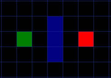
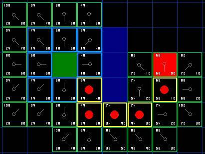
\(h(n)\)采用曼哈顿距离，即横纵向走的距离之和。
起始位置：绿色方块。
目标位置：红色方块。
障碍物：蓝色方块。
垂直、水平方向移动开销为10。
沿对角线移动开销为14。

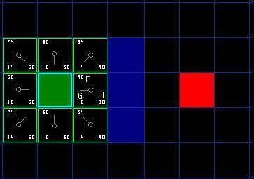
Open Set: 起点A。
将A相邻的8个节点中可走的加入Open Set，并将A设置为其父节点，然后移除。
将A加入Close Set。
从Open Set中选择一个节点：
- 选\(f(n)\)最小的。
  - \(h(n)\)采用曼哈顿距离，且忽略障碍物。

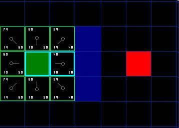
以此类推：

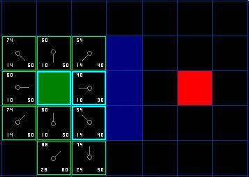
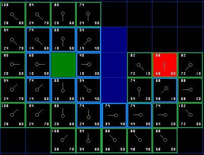
最终，从终点开始，向父节点移动到起点，即得到最优路径：

Hybrid-state A* Search²

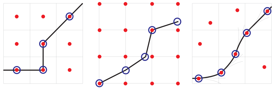
Left: A*, Center: D*, Right: Hybrid A*.

Input:
- an obstacle map.
- an initial state of the robot \(s_0 = (x,y,\theta)_0\).
- a goal state \(s_g = (x,y,\theta)_g\).
Output:
- a trajectory: \(s_0,s_1,\cdots,s_g\).
  - certain resolution: \(\Vert s_i - s_{i-1} \Vert \le \delta_s\).
  - safe, near-minimal in length, smooth and satisfies the kinematic constraints of the robot.
Algorithm process:
1. Use a variant of A* algorithm applied to the 3D kinematic state space of the robot.
  - Modify state update rule: captures continuous-state data in the discrete search nodes of A*.
  - Use a 4D search space \((x,y,\theta,r)\).
    - \(r = \{0,1\}\): the current direction of the motion (forward / reverse).
    - Add \(r\) to the path cost function:
      - penalties for driving in reverse.
        
        a multiplicative penalty that is applied to the length of segments driven in reverse.
      - for switching the direction of the motion.
        
        an additive penalty that is applied every time the robot switches directions.
  - Just as in conventional A*, the search space is discretized.
  - A graph is imposed on the grid with centers of the cells acting as neighbors in the search graph.
  - Unlike traditional A*:
    - Hybrid-state A* associates with each grid cell a continuous 3D state of the robot.
    - Initially, associate the current continuous state with the initial search node.
    - Pop a node from the open set.
    - Expand by applying several steering actions (max-left, no-turn, max-right) to the continuous state associated with the node.
    - Then, new children states are generated using a kinematic model of the robot.
  - Similar to Field D*:
    - Address the limitation of classical A* where only the centers of grid cells can be visited.
    - Field D* is limited to piecewise-linear paths.
    - Hybrid A* uses a continuous kinematic model when expanding the nodes, the paths produced are guaranteed to be drivable.
  - Heuristics:
    - Non-holonomic-without-obstacles.
      - Ignore obstacles.
      - Take into account the non-holonomic nature of the robot.
      - Compute the shortest path to the goal from every point in the 4D space \((x,y,\theta,r)\) in some discretized neighborhood of the goal.
      - Effect: It assigns high costs to search branches that approach the goal with the wrong heading.
    - Holonomic-with-obstacles.
      - Ignore the non-holonomic nature of the robot.
      - Use the obstacle map to compute the shortest distance to the goal by performing dynamic programming in 2D.
      - Effect: Give some path-cost (e.g. collision avoidance) imposed on the configuration space.
    - Use the maximum of the two heuristics for searching.
  - Analytic Expansions:
    - Forward search uses a discretized space of control actions (steering).
      - The search will never reach the exact continuous-coordinate goal state.
    - To address this issue and improve search speed:
      - Search with analytic expansions based on the Reed-Shepp model.
        
        A node in the tree is expanded by simulating a kinematic model of the robot for a small period of time.
        
        An additional child is generated by computing an optimal Reed-Shepp path from current state to the goal (obstacle-free environment).
        
        Because the implementation is more expensive than the regular forward node expansions.
        
        We can not apply the Reed-Shepp expansion to every node.
        
        Use a selection rule:
        
        Apply Reed-Shepp expansion to one of every N nodes.
        
        N decreases as a function of the cost-to-goal heuristic.
        
        More frequent analytic expansions will be applied as we get closer to the goal.
        
        Reed-Shepp path is then checked for collisions against the current obstacle map.
        
        The child node is only added to the tree if the path is collision-free.
      - The analytic extension of the search tree leads to significant benefits in both accuracy and planning time.
  - Variable resolution search:
    - Computational limitations of fixed resolution search:
      - Narrow passages might become untraversable if the resolution is too coarse.
      - Coarse resolution often leads to trajectories that oscillate around the optimal solution.
      - Computational efficiency.
    - The length of the trajectory arcs generated during the node expansion is determined by the amount of obstacle-free space around the node.
    - This allows us to take big steps forward in wide-open areas.
    - And, using a fine resolution in narrow passages.
2. Locally optimize the trajectory.
  - The paths produced are often suboptimal:
    - The paths contain unnatural swerves that require excessive steering.
  - Two-stage optimization producedure:
    1. Formulate a non-linear optimization program on the coordinates of the vertices of the path that improves the length and smoothness of the solution.
      - Using conjugate-gradient (CG) descent, a fast numerical-optimization technique.
      - But, does not change the path's discretization, still piecewise linear.
        
        This can lead to abrupt steering when used on a physical vehicle.
    2. Perform non-parametric interpolation on the output of the first stage using another iteration of a CG.
      - Minimize the curvature of the path.
      - Holding the original vertices fixed.
      - The interpolated paths have higher-resolution discretization.
      - Suitable for smooth control of the robot.

References

A*算法举例.

Stentz A . Optimal and efficient path planning for partially-known environments[C]// IEEE International Conference on Robotics & Automation. IEEE, 2002. ↩
D. Dolgov, S. Thrun, M. Montemerlo, and J. Diebel, “Path planning for autonomous vehicles in unknown semi-structured environments,” Int. J. Rob. Res., vol. 29, no. 5, pp. 485–501, 2010. ↩