Robust RL for UAV Control
Motivation
Quadrotor
- Applications:
dirty,dangerous,dulltasks.- Search and rescue missions.
- Various surveillance tasks.
- Acting as mobile nodes in communication networks.
- Quick delivery systems.
- Medical supplies.
- Some serious problem:
- How to hold algorithmically driven robots responsible for devastating actions?
- The lowered bar of entry to start warfare with cheaper robots to restrict the use of autonomous systems in warfare.
- Control:
- Lacking in stability compared to traditional designs.
- With smaller units resulting in
lower inertia momentsbeing moresusceptible to complex aerodynamical effects.
- With smaller units resulting in
- Require intricate control design in order to guarantee stable flight.
- Requirement on computational speed and accuracy.
- The dynamics are quick and non-linear.
- Requirement on computational speed and accuracy.
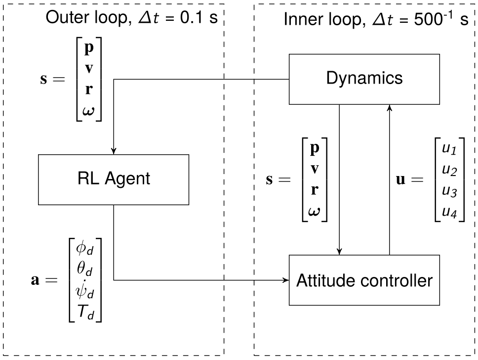
Control schemes:- Hierarchical:
- Lower level controllers:
- control of electrical signals to rotors.
- attitude controller.
- positional and altitude controller.
- Higher level controllers:
- path planning.
- problem solving.
- cooperation between humans or other units.
- Lower level controllers:
- Hierarchical:
Related works:- PID.
- LQR.
- \(H_\infty\).
- Sliding mode.
- MPC.
- RL:
- Attitude control.
- Positional control.
- S2R problem:
- Not transfer to real hardware and test on notably different simulated setups.
- Transferring successfully to real hardware but noticing some performance degradation.
- Implement methods of handling the S2R-gap and seeing improved transfer results.
None of these methods implemented the robust wersions of the underlying RL formulation.
- Lacking in stability compared to traditional designs.
S2R Transfer
![]()
- Sim-to-Reality (S2R) transfer in RL is a promising approach of
solving costly explorationin real systems.- Modifying the training such that
safety guaranteeson the training policy.- Safe RL.
- Modify the
objective functionorexploration policyare studied to minimize the risk costly exploration.
- Improving the
transferabilityof simulator-trained policies to actual systems.- Transfer Learning in RL.
- The agents performance on environments different than the environment trained in.
- Modifying the training such that
Problem:- S2R solves the costly exploration problem, but introduces
robustnessandgeneralizationconcerns. - The
generalizationof transferring policies from simulators to real systems. - Even if the agent finds an optimal policy inside the simulated environment, it is difficult to guarantee anything about the performance on the target environments.
- S2R solves the costly exploration problem, but introduces
Related works:- Making the S2R gap smaller:
- Making the simulated environment behave more closely to the target environment.
Accurate parameter estimationand more precise system indentification.Combine rollouts in real environmentand using the trajectories as feedback to improve the model behavior.Drawbacks:- The assumption is that there exists only one single target environment, but there may be
multiple possible target environments. - It is difficult or costly to gather information from the target environments.
- The assumption is that there exists only one single target environment, but there may be
- Consider random environments:
- Training on several model dynamics sampled from a priori parameter distribution representing the agents, which have been shown to better generalize to real systems.
Drawbacks:- The exact dynamics of the target environments is difficult to emulate.
- Robust control:
- Design controller to
tolerant to misspecificationsbetween models and real systems. - The controlled system in robust control is assumed to be
unknown but bounded. - The most popular robust controller designs is the \(H_\infty\) controller.
- Work with the
average bounded system optimizesinstead for the worst-case system. - Guarantee stability for all systems inside the bounds.
- Thus, it is popular for situation where robustness is required.
- Work with the
- Design controller to
- Making the S2R gap smaller:
Ideas:- Robust MDP.
- RL + Robust Control.
- Create agents with embedded
uncertaintyabout the simulated environment. - Training the agent in a simple environment and test on versions of the simulator with different environment parameters.
- Training environment.
- Target environments.
Results:- Agents with higher level of robustness outperformed the standard agents in these environments.
- The added
robustness increases generalityand can help when transferring policies from simulators to reality.
Method
Goal: Formulate a training method for RL agents to bridge the S2R gap.- Robust MDP:
Uncertainty setscan be expressed instate spaceinstead of probability distributions over the state space.
Framework
Model Uncertainty
- Express the uncertainty of the transition model through some uncertainty set in which all the possible transition models lie.
Inner Problem Definition
For discrete state space:
- The transition model can be expressed as
a set of transition matricesconsisting of finitely many elements of transition probabilities from and to each state given an action. - Define the
inner problemas:
For continuous state space:
- Remove the enumerability of the states.
- The
inner problemcan be transformed into:
The above inner problem expectation calculation is difficult to evaluate, since \(V^\pi\) in this setting will be a highly non-linear structure.
Then, make a huge simplifying assumption to this problem:
- In deterministic environments, the transition distributions \(P\) degenerate the expectation evaluation becomes trivial.
- Let \(P^U\) be a set of transition models with degenerate distributions \(p^u\) parameterized by states \(u\).
- Then, all probability density is located at \(u\).
Uncertainty Set
- View the uncertainty set as a possibility to
handle unmodelled behaviors(which are difficult to quantify).- Wind.
- Consider the sum of all of the unmodelled dynamics as some noise added to the transition dynamics.
- Reasons:
- The parameters of the system are not estimated.
- The model is crude and a lot of uncertainty would probably come from
unmodelled dynamics. - The uncertainty modeling becomes simpler to implement.
The deterministic model can be seen as a degenerate distribution:
- Parameterized by the point in state space.
- The entirely of the probability density is located.
- The uncertainty set can be
reinterpreted as a set over the state spaceinstead over transition dynamics.
Consider an uncertainty set around each observed state \(s\) in a trajectory:
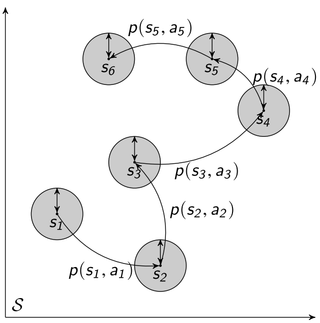
where \(U(s)\) is a priori asserted uncertainty set.
Let \(U(s)\) as \(L_2\) spheres in the state space:
\[U_\rho(s) = \{ u\in \mathbb{R}^S \vert \lVert u \rVert_2 < \rho \},\]where \(\rho\) is the size of uncertainty, can be viewed as radius.
Solving Inner Problem
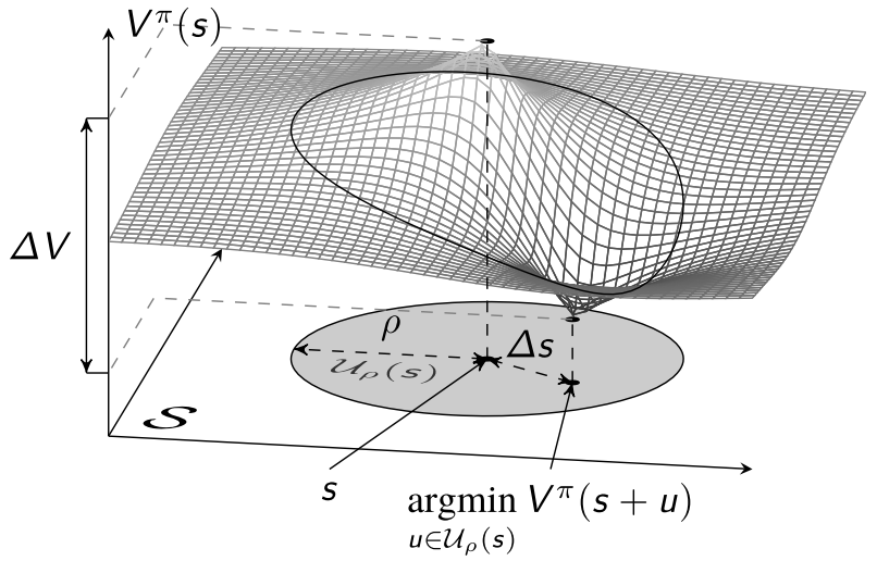
Minimize the value function given the uncertainty set:
\[\min_{u\in U}V_\phi^\pi(s+u).\]Algorithm:
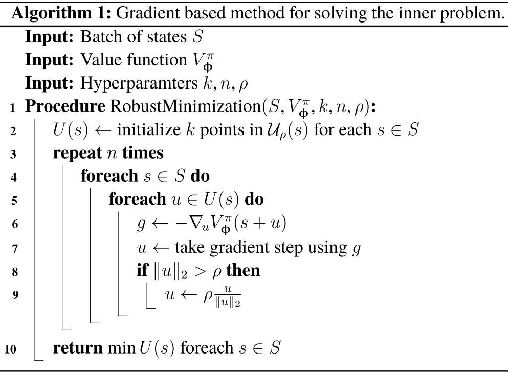
- Hyperparameters:
- \(k\) for width, controls how many points are computed in parallel.
- \(n\) for depth.
- \(n\) controls how many gradient steps are taken before we assume convergence.
Robust PPO
- Replace training targets using Bellman equations with the
robust Bellman equationsinstead.
Estimate \(\hat{R}\) and \(\hat{A}\)
- Using truncated \(n\)-step TD to estimate.
- Apply a decaying scheme for parameter \(\lambda\).
- In order to reduce computations, handle episodic tasks, reduce reliance on too long traces.
Define the \(n\)-step robust returns for a trajectory:
Define the \(n\)-step robust advantage estimates:
Using Truncated TD(\(\lambda\)) to estimate \(\hat{R}_t\):
\[\begin{aligned} \hat{R}_t^{\rho TTD(\lambda,N)} & = (1-\lambda)\hat{R}_t^{\rho(1)} + \lambda\left( (1-\lambda)\hat{R}_t^{\rho(2)} + \lambda(\cdots) \right) \\ & = (1-\lambda)\sum_{n=1}^{N-1}\lambda^{n-1}\hat{R}_t^{\rho(n)} + \lambda^{N-1}\hat{R}_t^{\rho(N)}. \end{aligned}\]Using Truncated GAE(\(\lambda\)) to estimate \(\hat{A}_t\):
\[\hat{A}_t^{\rho TGAE(\lambda,N)} = (1-\lambda)\sum_{n=1}^{N-1}\lambda^{n-1}\hat{A}_t^{\rho(n)} + \lambda^{N-1}\hat{A}_t^{\rho(N)}.\]Algorithm:

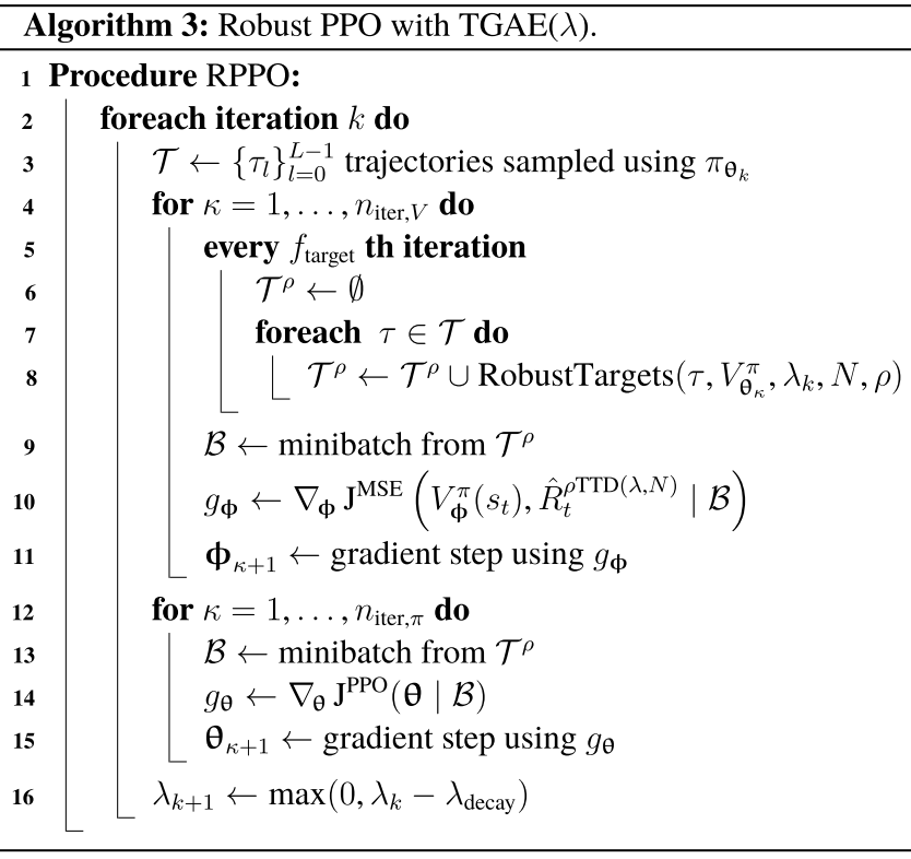
Algorithm of Robust PPO
- Incorporate a decaying scheme for the trace parameter \(\lambda\):
- High \(\lambda\) greatly improves training in early iterations when the critic network has not yet converged to a useful approximator.
- \(\lambda=0\) is needed in order to represent the correct robust equations for training targets.
- Using a
linear decaying scheme, \(\lambda_{decay}\) controls the speed at which the trace reaches zero.
Robust TD-error to fit the value function approximator:
Robust advantage estimation to fit the policy function:
Robust PPO for UAV positional control
State Input
\[(p_t^e, v, \Theta, \omega, e_{p_t}, e_{v_t}, e_{\sigma_t}).\]- \(p_t^e = p_t^g - p_t\).
Action Output
\[(\phi_d,\theta_d,\dot{\psi}_d, T_d).\]- Remove yaw rate, set it to a constant \(\dot{\psi}_d = 0\).
- Rescale the possible range for the remaining action outputs:
- Angles \(\phi_d, \theta_d\) range: \([-10^\circ,10^\circ]\).
- Thrust \(T_d\) range: \([10000,65535]\).
- Normalize the action: \([-1,1]\).
Environment terminal time
- The agent is more interested in the behavior before reaching the goal position.
- Then, episode is needed.
- Add a time limit \(T_{limit}\).
- In order to let the agent see initial states more often.
- End the episode when:
- A failure state.
- \(V(s_T) = -1\).
- Maximum number of interactions has been reached (limit time).
- \(V(s_T) = V(s_T)\).
- A failure state.
Neural Networks
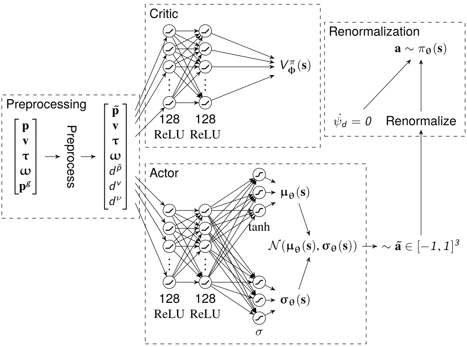
- MLP.
- Critic network:
- The output layer is a simple linear layer with one output.
- Actor network:
- Two output layers representing parameters for Gaussian distributions:
- Mean values \(\mu_\theta(s)\in [-1,1]\) with
tanhactivation function. - Standard deviations \(\sigma_\theta(s)\in[0,1]\) with
sigmoidactivation function, in order to impose limits on the variance of the distribution.
- Mean values \(\mu_\theta(s)\in [-1,1]\) with
- Two output layers representing parameters for Gaussian distributions:
Regularization
Definition:
- Regularization is a general term for
modification to objective functionsto guide optimization in ill-posed problem. - In ML, it is widely used to
combat overfitting.
Formulate the regularization to objective function as:
\[J(\theta) + \sum_{i=1}^I \beta_i l_i(\theta),\]where \(\beta_i\) is the regularization weight to set the strength of the regularization term.
Using regularization in robust PPO:
- Entropy regularization for actor network.
- Trade-off between exploration and exploitation.
Exploitation: using current knowledge to collect high rewards.Exploration: searching the policy space to potentially find better policies to follow.
- Usually resolved with heuristical methods.
Entropycan be seen as the uncertainty of a distribution.- \(H(p) = -\int_X p(x)\log(x)dx\).
- Entropy regularization: \(l_H(\theta) = \mathbb{E}_{\pi_\theta}[H(\pi_\theta(a_t\vert s_t))]\).
- Prevent too deterministic policies.
- Encourage a higher level of exploration in the on-policy setting.
- Trade-off between exploration and exploitation.
- \(L_1\) regularization for both actor and critic networks.
- Tend to favor sparsity in the weight vector.
- Reduce the model complexity.
- Tend towards simpler models by pruning model weights.
- Does not impact the original objective significantly enough.
- Parameter weights regularization:
- For actor network weights: \(l_{L_1}(\theta) = \lVert \theta \rVert_1\).
- For critic network weights: \(l_{L_1}(\phi) = \lVert \phi \rVert_1\).
Simulation
Implementation
- Simulator: RLlib framework.
- Distribute training across multiple processes.
- Parallelize the agent rollouts.
- Wrapper: OpenAI Gym API.
- NNs: Pytorch.
- Gradient method: Adam.
Training
- Training multiple agents with values of robust radius \(\rho\in[0.001,1]\).
- Compare these agents to the baseline of a regular PPO agent with \(\rho=0\).
Evaluation
- Test the robustness of the policy in
target environments.- Different to the training environment.
- Target environments:
- Different quadrotor mass: \(\Delta m\in [0.7,1.3]\).
- Different motor coefficients:
- Change the coefficients of one of the motors in the model, corresponding to damaged or worn.
- The motors are modeled with a set of polynomial coefficients mapping digital driver values to physical values \([c_T,b_T,a_T,b_\omega,a_\omega,b_\psi,a_\psi]\).
- Multiply these coefficients by a factor: \(\Delta \lambda \in [0.3,1]\).
- Different PID tuning:
- PID parameters of internal attitude controller.
- Multiply a factor \(\Delta K_p\in[0.1,1.9]\) to the proportional gain \(K_p\) of the roll and pitch controllers: \([PID_\phi.K_p, PID_\theta.K_p, PID_{\dot{\phi}}.K_p, PID_{\dot{\theta}}.K_p]\).
- Performance metric:
- Use the episodic average step reward measured from an episode: \(\bar{r}(\tau) = \frac{\sum_{k=0}^{T-1}r_t}{T}\).
- Robust performance:
- Remove the stochastisity in the policy, picking the
mean value\(\mu_\theta\) of the policy distribution.
- Remove the stochastisity in the policy, picking the
Results
- Convergence seems clear for agents with lower values of \(\rho\), but asymptotic performance does taper off as the radius grows.
- Performance dropping after \(\rho = 0.1\).
- Robustness of the agents:
- Running each agent in different target environments.
- The robust agents outperforms the nominal in the more extreme environment differences.
- The robust agents do not suffer from an immediate performance drop in the nominal environment.
- More robust agents performs similar to slightly better than the non-robust agent for environments close to the nominal.
- Reduce the oscillations and static errors.
Static errors:- especially in the \(z\)-axis.
- Static errors are widely understood in the control theory where controllers with
integral action.- Integral action is the most
non-Markovianpart of controllers.
- Integral action is the most
Future Work
- Robust MDP for continuous control
- Deterministic systems.
- Moving all the uncertainty into the second order uncertainty sets (on state observations).
- Non-deterministic systems.
- Require measurements on probability distributions.
- Consider other uncertainty sets on state observations.
- Deterministic systems.
- Robustness of other RL algorithms
- DQN
- DDPG
- SAC
- RL for UAV control
- End-to-end control.
- Static errors.
- Handle via integral action.
- Extend the state space to include the sum of error signals.
- Increase the dimensionality of the state space and the search space for policies.
References
- L. Bjarre, “Robust Reinforcement Learning for Quadcopter Control,” 2019.