Trajectory Planning for Aggressive Maneuvers
Trajectory Planning
- Generate
dynamically feasibletrajectories that will take the quadrotor to its destination. - Aggressive maneuvers:
- Trajectory over the narrow window gap.
- Slalom path.
Trajectory over the narrow window gap

Quadrotor model
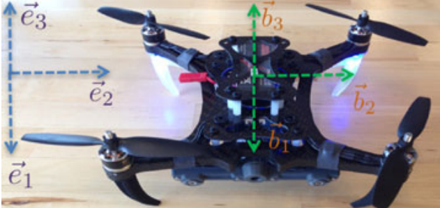
Where \(\mathbf{R} = [\mathbf{b}_1,\mathbf{b}_2,\mathbf{b}_3]\).
Trajectory generation
According to differential flatness property:
According to quadrotor model:
\[F = m\Vert \ddot{\mathbf{p}} + g\mathbf{e}_3\Vert,\] \[\mathbf{b}_3 = \frac{\ddot{\mathbf{p}} + g\mathbf{e}_3}{\Vert \ddot{\mathbf{p}} + g\mathbf{e}_3\Vert},\] \[\mathbf{b}_2 = \frac{\mathbf{b}_3\times \mathbf{b}_C}{\Vert \mathbf{b}_3\times\mathbf{b}_C\Vert},\]where \(\mathbf{b}_C = [\cos\psi, \sin\psi,0]\) is the projection of \(\mathbf{x}_b\) to \(\mathbf{x}_W\times\mathbf{y}_W\) plane.
Then,
\[\mathbf{b}_1 = \mathbf{b}_2\times\mathbf{b}_3.\]The derivative of \(m\dot{\mathbf{v}} = \mathbf{R}F \mathbf{e}_3 - mg\mathbf{e}_3\) is:
\[m\mathbf{p}^{(3)} = - F \dot{\mathbf{R}}\mathbf{e}_3 - \dot{F}\mathbf{R}\mathbf{e}_3 = -F\mathbf{R}\hat{\omega}\mathbf{e}_3 - \dot{F}\mathbf{b}_3,\] \[\dot{F} = \mathbf{b}_3\cdot m\mathbf{p}^{(3)}.\]Then, determine the first two terms of the angular body rates:
\[\begin{bmatrix} \omega_x \\ \omega_y \end{bmatrix} = \frac{m}{F}\begin{bmatrix} -\mathbf{b}_2^T \\ \mathbf{b}_1^T \end{bmatrix}\mathbf{p}^{(3)}.\]Decomposing \(\mathbf{R}\) by the euler angles:
\[\omega_z = \omega_x\tan\theta + \frac{\cos\phi}{\cos\theta}\dot{\psi}.\]Similarly, we can obtain the angular acceleration.
Trajectory optimization
The control inputs can be computed in terms of the flat outputs and their derivatives:
- The \(4^{th}\) derivative of position appears in the control inputs.
- The \(2^{th}\) derivative of the yaw appears in the moments.
Minimize the following cost function:
\[L = \int_{t_0}^{t_f} \left\Vert\frac{d^4\mathbf{p}(t)}{dt^4}\right\Vert^2 dt + \left\Vert\frac{d^2\psi(t)}{dt^2}\right\Vert^2 dt.\]Constraints:
- Equality constraints:
- Guarantee during the trajectory the continuity of position and its derivatives.
- Specify a constraint at a desired time.
- Inequality constraints:
- \(\mathbf{v}_{max}\).
- \(m\Vert\ddot{\mathbf{p}}+g\mathbf{e}_3\Vert \le F_{max}, \forall t\in [t_0,t_f]\).
- \(F_{max} = \sum_{j=1}^4 f_j^{max} = 4k_f \left(\omega_{max}^m\right)^2\).
- \(f\left( \mathbf{p}^{(3)},\ddot{\mathbf{p}},\dot{\psi} \right) \le \omega_{max}, \forall t\in[t_0,t_f]\).
- \(f\left( \mathbf{p}^{(4)},\mathbf{p}^{(3)},\ddot{\mathbf{p}},\dot{\psi},\ddot{\psi} \right) \le \tau_{max},\forall t\in[t_0,t_f]\).
- \(\tau_{max} = l(\omega_{max}^m - \omega_{min}^m)\).
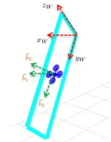
Trajectory through a narrow gap
Identify the window gap using a planar homography algorithm, output:
- \(\mathbf{R}_w = [\mathbf{x}_w,\mathbf{y}_w,\mathbf{z}_w]\), the rotation of the window gap w.r.t. the initial robot frame \(b\).
- \(\mathbf{p}_w\), the translation of the window gap w.r.t. body frame \(b\).
The quadrotor can only traverse the window gap such that the main body plane is orthogonal to the window planar surface defined by \(\mathbf{y}_w\times\mathbf{z}_w\).
Define the traversing window point as \(\mathbf{p}_w\), enforce the orientation \(\mathbf{R}_w\) at the gap with the following acceleration constraint:
\[\mathbf{a}_{w_{des}} = \mathbf{R}_w^T \mathbf{a}_w - g\mathbf{e}_3,\]where \(\mathbf{a}_w = a\mathbf{e}_3\).
Slalom path
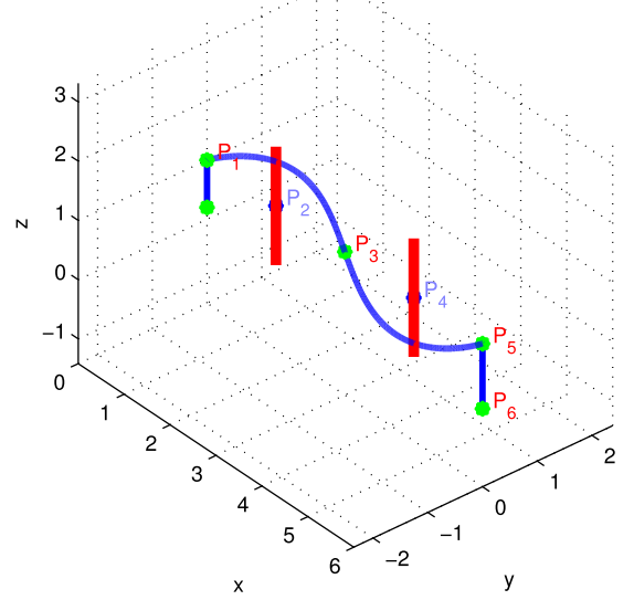
Increase degree of difficulties in term of acceleration, velocity and attitude angles.
Assume to know the obstacles’ locations (\(P_2,P_4\)) w.r.t. the quadrotor’s starting position.
The obstacle’s position imposes some constraints on the planned trajectory.
Consider a set of virtual waypoints \(P_{v_i}(P_{v_{i_x}}, P_{v_{i_y}},P_{v_{i_z}})\) located at the obstacle positions and their corresponding times instants \(t_{v_i}\).
Impose in the QP problem a bound on each of the dimension around the obstacles’ positions as:
\[\begin{aligned} p_x(t) & \ge P_{v_{i_x}} + \epsilon_x, \\ p_y(t) & \ge P_{v_{i_y}} + \epsilon_y, \\ p_z(t) & \ge P_{v_{i_z}} + \epsilon_z, \\ \forall t & \in (t_{v_i} - \delta, t_{v_i} + \delta), \end{aligned}\]where
- \(\delta\) is a time interval.
- \(\epsilon_x,\epsilon_y,\epsilon_z\) indicate the thresholds the quadrotor’s center should respect to be safe.
References
- G. Loianno, C. Brunner, G. McGrath, and V. Kumar, “Estimation, Control, and Planning for Aggressive Flight with a Small Quadrotor with a Single Camera and IMU,” IEEE Robot. Autom. Lett., vol. 2, no. 2, pp. 404–411, Apr. 2017.