Trajectory Optimization for Quadrotors

Motivation

Trajectory planning \(\to\) Navigation

Quadrotors rely on robust and efficient trajectory planning for safe yet agile autonomous navigation in complex environments.

High-quality motions subject to the precisely incorporating:

• dynamics
• smoothness
• safety

Few of the existing trajectory planning or optimal control can guarantee high-frequency online planning while also consider general constraints on dynamics for quadrotors.

For high-performance planning, challanges:

• Ensure motion safety.
• Nonlinearity of vehicle dynamics.
• High-quality motions.
• Sparse representation for trajectories lack an effective way to optimize the temporal profile.

Reliable motion planning: requires that all dynamic constraints satisfied at a high resolution.

Related work

Existing trajectory planning approaches have yet to emerge a complete framework to accomplish high-frequency large-scale planning while:

• incorporating user-defined continuous-time constraints on state and control.
• high-quality motion subject to complex dynamic constraints.
• in the time-critical flights of a lightweight quadrotor.

Differential flatness

This property makes it possible to recover the full state and input of a flat system from finite derivatives of its flat outputs.

• Kumar, 2011:
  • utilize the flatness to generate trajectories that meet differential constraints.
  • compute the feedforward term of a tracking controller.
• UZH, 2018:
  • consider more complicated system dynamics with aerodynamic effect to design a high-speed flight controller.
  • present the flatness of the quadrotor system subject to the rotor drag.
• Mu, 2019:
  • investigate underactuated quadrotors with tilted propellers.
  • prove that the flatness holds for a wide range of tricopters, quadrotors and hexacopters.

Flatness is beneficial to trajectory generation and tracking in that the reference state and input can be algebraically computed.

Sampling-based Motion Planning

Possess the nature of exploration and exploitation in the solution space.

It well suits the seeking for global solutions of non-convex problems where the complexity mainly originates from the configuration space.

• Probabilistic Roadmap (PRM), 1996:
  • constructs an obstacle-free graph from randomly sampled feasible vertices in a static configuration space for multiple queries of shortest paths.
• Rapidly-exploring Random Tree (RRT), 1998:
  • incrementally builds a tree by online sampling based on a single query’s information.
• PRM\(^*\) and RRT\(^*\), 2011:
  • analyze the asymptotic optimality conditions for sampling-based algorithms.
  • These variants ensure the convergence to the globally optimal solution as the sample number goes to infinity.

The optimal sampling-based planner is promising, albeit time-consuming, when the robot has many Degrees of Freedom (DoFs) and the configuration space is highly nonconvex.

Optimization-based Motion Planning

Focus on local solutions of motion planning problems where objectives or optimality criteria are specified.

They are often built on specific environment pre-processing methods such that obstacle information is encoded into the optimization as objectives or constraints.

Trajectory optimization, viewed as an optimal control problem, general-purpose solvers:

• ACADO, 2011
• GPOPS-II, 2014
  • The original optimization is often discretized and transcribed into a Nonlinear Programming (NLP).
    • solved by SNOPT or IPOPT.

However, robotic motion planning may impose:

• hard-to-formulate constraints
• nonsmoothness
• even integer variables

General-purpose methods often take a relatively long computation time.

• inappropriate for time-critical applications.

Contributions

• Present an optimization-based framework for quadrotor trajectory planning subject to:
  • geometrical spatial constraints.
    • Smooth maps are utilized to exactly eliminate geometrical constraints in a lightweight fashion.
  • user-defined dynamic constraints.
• Design a lightweight and flexible optimization framework to meet various motion requirements based on a novel trajectory class.
• A novel trajectory representation built upon the novel optimality conditions for unconstrained control effort minimization.
• MINCO (Minimum Control) is designed to directly control the spatial and temporal profile of a trajectory.
• The framework bridges the gaps among solution quality, planning frequency, and constraint fidelity for a quadrotor with limited resources and maneuvering capability.
• Efficiency, optimality, generality and robustness.
  • Safely and agilely maneuvers through several narrow tilted gaps sequentially.
  • Real-time interactions with a gap that is arbitrarily placed.
• Code and video: http://zju-fast.com/gcopter.

Method

Differential Flatness

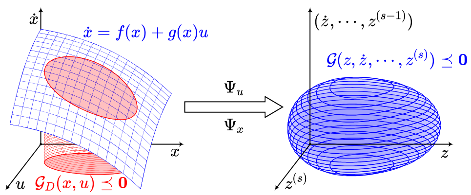
Dynamic system:

where

• \(f:\mathbb{R}^n \mapsto \mathbb{R}^n\).
• \(g:\mathbb{R}^n \mapsto \mathbb{R}^{n\times m}\).
  • The map \(g\) is assumed to have rank \(m\).
• State: \(x\in \mathbb{R}^n\).
• Input: \(u\in \mathbb{R}^m\).

Define a flat output \(z\in\mathbb{R}^m\), \(x\) and \(u\) can both be parameterized by finite derivatives of \(z\):

where

• \(\Phi_x:(\mathbb{R}^m)^{s-1}\mapsto \mathbb{R}^n\).
• \(\Phi_u:(\mathbb{R}^m)^s\mapsto \mathbb{R}^m\).

Direct Optimization in Flat-output Space

Flat output:

Trajectory:

Spatial constraints:

• trajectory smoothness
  • adopt the quadratic control effort with time regularization as the cost functional over \(z(t)\).
• feasibility
  • constraints coming from the configuration space.
    • a collision-free motion: \(z(t)\in \mathcal{F}, \forall t\in[0,T]\).
      • \(\mathcal{F}\) is the concerned obstacle-free region in configuration space.
  • other constraints on state and control of system dynamics
    • actuator limits
    • task-specific constraints
    • All user-defined constraints are denoted by \(\mathcal{G}_D(x(t),u(t))\le \mathbf{0},\forall t\in[0,T]\).
      • \(\mathcal{G}(z(t),\dot{z}(t),\cdots,z^{(s)}(t))\le\mathbf{0},\forall t\in[0,T]\).

Convert to optimization problem

Where

• \(\mathbf{W}\in\mathbb{R}^{m\times m}\) is a diagonal matrix with positive entries.
• \(\rho:[0,\infty)\mapsto [0,\infty)\) the time regularization term.
• \(\bar{z}_o\in\mathbb{R}^{ms}\) the initial condition.
• \(\bar{z}_f\in\mathbb{R}^{ms}\) the terminal condition.
• \(\mathcal{G}\): the continuous-time nonlinear constraints.
• \(\mathcal{F}\): nonconvex set constraint.

For the time regularization \(\rho\)

• it trades off between the control effort and the expectation of total time.

where \(b_{M_T}\) is strictly positive.

Common choices:

Where \(T_\Sigma\) is the expected time.

Also, \(\rho\) can be defined to strictly fix the total time:

For nonlinear constraints \(\mathcal{G}\)

• they are required to be \(C^2\) (i.e. twice continuously differentiable).

For the feasible region \(\mathcal{F}\) in the configuration space

where \(P_i\) is a closed convex set, with the following property:

1. locally sequential connection is assumed on these convex sets: \(\begin{cases} P_i \cap P_j = \varnothing & if \vert i-j\vert = 2, \\ Int(P_i\cap P_j) \neq \varnothing & if\vert i-j \vert \le 1, \end{cases}\) where \(Int(\cdot)\) is the interior of a set.
2. consider that each \(P_i\) is a closed \(m\)-dimensional ball: \(P_i^B = \left\{ x\in\mathbb{R}^m \big\vert \Vert x - o_i\Vert_2 \le r_i \right\}.\)
3. or, a bounded convex polytope described by its \(H\)-representation: \(P_i^H = \left\{ x\in\mathbb{R}^m \big\Vert A_i x\le b_i \right\}.\)

Multi-stage Control Effort Minimization

• Without functional constraints.
• Propose esay-to-use optimality conditions
  • necessary and sufficient.
• Leveraging the conditions:
  • the optimal trajectory is directly constructed in linear complexity of time and space.
  • without evaluating the cost functional explicitly or implicitly.
  • A novel trajectory class along with linear-complexity spatial-temporal deformation is designed to meet user-defined objectives in various trajectory planning scenarios.

Unconstrained Control Effort Minimization

• The spatial constraints \(\mathcal{F}\) and functional constraints \(\mathcal{G}\) are not considered temporarily.
• The intermediate points and time vector are given in advance.
• Consider the \(M\)-stage control effort minimization for a chain of \(s\)-integrators.

• The interval \([t_0,t_M]\) is split into \(M\) stages by \(M+1\) fixed time stamps.
• Some derivatives of the flat output are fixed as \(\bar{z}_i\in \mathbb{R}^{md_i}\) at \(t_i\), the end of each stage.
• \((d_i-1)<s\) is the highest order of specified derivatives.

Optimality Conditions

Transform the above problem from the Lagrangian form into Mayer form by state augmentation:

where the new state \(y\in\mathbb{R}^{ms+1}\) augmented by a scalar \(\tilde{y}\in\mathbb{R}\).

The augmented system:

Hybrid Maximum Principle

Optimality Conditions

• A trajectory is optimal, if and only if the following conditions are satisfied:
  • The map \(z^*(t): [t_{i-1},t_i]\mapsto \mathbb{R}^m\) is parameterized as a \(2s-1\) degree polynomial for any \(1\le i\le M\).
  • The boundary conditions.
  • The intermediate conditions.
  • \(z^*(t)\) is \(\bar{d}_i-1\) times continuously differentiable at \(t_i\) for any \(1\le i<M\), where \(\bar{d}_i = 2s-d_i\).

Minimization Without Cost Funcional

• Optimality conditions provide a straightforward way to compute the unique optimal trajectory.
• The computation even does not require explicit or implicit evaluation of the cost functional or its gradient.

Consider an \(m\)-dimensional trajectory, the \(i\)-th piece is denoted by an \(N=2s-1\) degree polynomial:

where

• \(\mathbf{c}_i\in\mathbb{R}^{2s\times m}\) is the coefficient matrix of the piece.
• \(T_i\) is the piece time.
• \(\beta(t) = [1,t,\cdots,t^N]^T\) is the natural basis.

Define the coefficient matrix \(\mathbf{c}\in\mathbb{R}^{2Ms\times m}\):

Define the time vector \(\mathbf{T}\in\mathbb{R}^M\):

Then, the trajectory \(p:[0,T]\mapsto \mathbb{R}^m\) is parameterized as:

where \(t_i = \sum_{j=1}^i T_j\), and \(T = t_M\).

MINCO Trajectories with Spatial-Temporal Deformation

• The safety of a flight trajectory is dominated by its spatial profile.
• The dynamic limits are dominated by its temporal profile.

Then, divide parameters of a trajectory into two groups:

• intermediate points that the trajectory should pass through.
• the time vector for different pieces of the trajectory.

All coefficients of a polynomial spline can be generated from the conditions.

The trajectory naturally belongs to a minimum control effort class, which is named by MINCO.

Define the intermediate points as \(\mathbf{q} = (q_1,\cdots,q_{M-1})\), where \(q_i\in \mathbb{R}^m\).

The MINCO trajectory class is defined as:

All the trajectories in \(\mathcal{T}_{MINCO}\) are compactly parameterized by only \(\mathbf{q}\) and \(\mathbf{T}\).

• Adjusting \(\mathbf{q}\) yields the spatial deformation, such that the trajectory is collision-free.
• Adjusting \(\mathbf{T}\) yields the temporal deformation, such that the dynamic limits are satisfied.

Define the user-defined objective on a trajectory as a \(C^2\) function \(F(\mathbf{c},\mathbf{T})\) with available gradient:

• The gradient \(\partial H/\partial \mathbf{q}\) and \(\partial H/\partial \mathbf{T}\) are needed for a high-level optimizer to optimize the objective.
• The gradient propagation is done in \(O(M)\) linear time and space complexity.

Geometrically Constrained Flight Trajectory Optimization

An unified framework is provided for flight trajectory optimization with different:

• time regularization \(\rho(T)\).
• spatial constraints \(\tilde{\mathcal{F}}\).
• continuous-time constraints \(\mathcal{G}\).

The spatial-temporal deformation is utilized to meet various feasibility constraints while maintaining the local smoothness.

For geometrical constraints:

• an elimination method is proposed such that the spatial-temporal deformation is free from the Combinatorial Difficulty of inequalities.

For continuous-time constraints on the trajectory:

• a time integral penalty functional is proposed to ensure the feasibility under a prescribed resolution without sacrificing the scalability.

An efficient and flexible gradient propagation turns the constrained optimization into an unconstrained one which can be reliably solved.

Temporal Constraint Elimination

The time regularized control effort can be written as:

where

• \(J_q(\mathbf{q},\mathbf{T}):= J_c(\mathbf{c}(\mathbf{q},\mathbf{T}),\mathbf{T})\).
• \(J_c(\mathbf{c},\mathbf{T})\) is the control effort of a polynomial spline.

Two implicit temporal constraints do harm to the optimization process:

1. \(J_q(\mathbf{q},\mathbf{T})\) is defined on \(\mathbb{R}^M\), which requires the strict positiveness of each entry in \(\mathbf{T}\).
2. \(\rho = \rho_f\) adds an extra linear constraint on \(\mathbf{T}\).
   • make the feasible region much more limited.

Propose a diffeomorphism based method to eliminate the temporal constraints for both kinds of time regularization.

Consider the domain for \(\rho_f\) as:

The set \(T_f\) is diffeomorphic (微分同胚) to \(\mathbb{R}^{M-1}\).

An element in \(\mathbb{R}^{M-1}\) is \(\tau = (\tau_1,\cdots,\tau_{M-1})\).

The \(C^\infty\) diffeomorphism is given by the map:

Using the diffeomorphism, optimize the cost function \(J\) directly in the whole \(\mathbb{R}^{M-1}\) or \(\tau\).

TODO

Spatial Constraint Elimination

The geometrical constraints \(\tilde{\mathcal{F}}\) should also be enforced to ensure a collision-free trajectory.

• requires the whole continuous-time trajectory to be contained by an union of obstacle-free geometrical regions.
  • intermediate points are sequentially assigned to these convex regions so that the trajectory approximately lies in free space.
  • the whole trajectory is contained by the geometrical constraints under any given relative resolution.

Consider the constraint \(q\in P\), where

• \(q\in\mathbb{R}^n\) is a point.
• \(P\subset\mathbb{R}^n\) is a closed ball set or a closed convex polytope.
  • \(P^B = \left\{ x\in\mathbb{R}^n\vert \Vert x-o\Vert_2\le r \right\}\).

Propose a spatial constraint elimination method to preserve the exact description of the hard constraints.

1. Utilize a smooth surjection to map \(\mathbb{R}^n\) to \(P^B\).
2. The optimization over the unconstrained Euclidean space implicitly satisfying the constraint described by \(P^B\).

TODO

Time Integral Penalty Functional

Trajectory Optimization via Unconstrained NLP

• The optimal trajectory parameterization is generally hard to known.
• Propose a lightweight relaxed trajectory optimization via an unconstrained NLP.

Define the relaxation as:

where

• \(J\) is the time-regularized control effort for \(\mathcal{T}_{MINCO}\).
• \(I_\Sigma\) is the quadrature of penalty functional for splines.

Advantages:

• use compact parameterization.
• constraint elimination by variable transformations.
• softened penalty for continuous-time constraints.
• Any task-specific requirement on a trajectory can be added into the framework.

Experiments

Large-Scale Unconstrained Control Effort Minimization

Trajectory Generation within Safe Flight Corridors

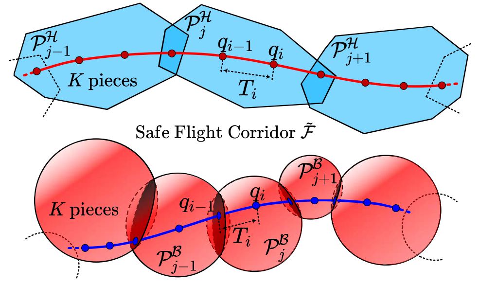
• Optimizing trajectories within 3D Safe Flight Corridors (SFCs) is widely adopted in various applications.
  • An SFC is generated by the front end of a motion planning framework as an abstraction of the concerned configuration space.
    • Polyhedron-shaped or Ball-shaped.
    • Obtained through a frond end such as
      • RILS algorithm
      • IRIS
      • Sphere Flipping based method
      • Safe-region RRT\(^*\) Expansion algorithm
  • Optimizing dynamically feasible trajectories within SFCs is taken as a back end of the framework.

SE(3) Motion Planning in Quotient Space

• Safe motion will not exist for narrow spaces unless a quadrotor agilely adjusts its rotation to avoid unnecessary collisions.
• Motion planning in \(SE(3) = \mathbb{R}^3\times SO(3)\).
  • A feasible pose for the body at least contains a feasible translation for a dimensionless point.
  • Subspace \(\mathbb{R}^3\) is often referred to as a Quotient Space.
  • Consider the rotational feasibility based on an translational trajectory.

Agile Flight through Narrow Windows

• The poses of narrow windows and the quadrotor are all provided by external motion capture system running at 100Hz.
• Run the planner on an offboard computer such that a human operator can arbitrarily choose the goal position for robustness testing.
• Trajectory tracking.
• Actual maximum speed and body rate reach \(4.1m/s\) and \(8.4m/s\), respectively.

Challenges:

• Large roll angles of the windows.
• Short distance between consecutive windows.
• Small acceleration/deceleration space.
• Limited maneuvering capability of the quadrotor.

References

• Z. Wang, X. Zhou, C. Xu, and F. Gao, “Geometrically Constrained Trajectory Optimization for Multicopters,” Feb. 2021.