Trajectory Planner for Agile Flights in Unknown Environments
Motivation
- The unlimited applications of quadrotor autonomous navigation in unknown environments:
- aerial surveying and inspection.
- search and rescue.
These applications are often reduced to low-speed flights due to:
- The limitations and low rates of the mappers and planners.
- The inherent non-convexity of the path planning optimization problem.
A real-time planner that runs onboard and plans fast and safe trajectories in completely unknown environments is still an open problem.
Problem
Planning high-speed trajectories for quadrotors in unknown environments:
- requires extremely fast algorithms able to
solve the trajectory generation problemin real-time. react quicklyto the changing knowledge of the world.- guarantee
safetyat all times.- Obtained by having a local planner that plans a trajectory with a final
stopcondition in the free-known space. - However, this decision
leads to slow and conservative trajectories.
- Obtained by having a local planner that plans a trajectory with a final
Contributions
| Planner | Dynamics | Environment | Planning Space | Planning Time | Solver | \( v_{max} \) |
|---|---|---|---|---|---|---|
| Global | Full state nonlinear model | Known | Everywhere | \(7 min\) | GPOPS-II | - |
| Global + Local | Triple integrator | Unknown | \(F\) | \(5\sim 40 ms\) | CVXGEN | \(3.5m/s\) |
| Global + Local | Triple integrator | Unknown | \(F\cup U\) | \(20\sim 65 ms\) | CVXGEN | \(7.8m/s\) |
Full Dynamics Trajectory Optimization
- Environment is known.
- Not real-time.
- Global optimal.
Real-time Planning
- Real-time.
- Environment is unknown.
- Safe but slow.
FASTER
- Global planner:
JPS. - Reformulate the optimization problem of the
local planneras aMixed Integer Quadratic Program (MIQP).- Use differential flatness.
- Use a convex decomposition of the space.
Safety guaranteesare ensured by always having a feasible, safe back-up trajectory in the free-known space at the start of each replanning step.
Trajectory Optimization with Nonlinear Model
Contributions
- Formulation of the
planning problemas anoptimal control problem, consider the full nonlinear dynamics of the quadrotor. - Implement the formulation in a cluttered drone racing environment to find the
optimal trajectory.- Assume that the environment is completely known.
- Solution for the
optimal control problemis obtained using:- Solver: GPOPS-II.
- sparse nonlinear programming
- hp-adaptive pseudospectral method
- Matlab
- C++
- Solver: GPOPS-II.
- Video: https://www.youtube.com/watch?v=-YY_0Ib-o_4.
Quadrotor dynamics

Brushless Motor Model
\[\begin{aligned} f_i & = k\omega_i^2, \\ \tau_i & = \pm b\omega_i^2. \end{aligned}\]Thrust and Torques
\[\begin{bmatrix} T \\ \tau_\phi \\ \tau_\theta \\ \tau_\psi \end{bmatrix} = \begin{bmatrix} \sum_{i=1}^4 f_i \\ lk(\omega_2^2 - \omega_4^2) \\ lk(-\omega_1^2 + \omega_3^2) \\ \sum_{i=1}^4 \tau_i \end{bmatrix}.\]Control inputs
\[\mathbf{u} = [T \quad \tau_\phi \quad \tau_\theta\quad\tau_\psi]^T.\]State equations
- Newton-Euler.
Environment
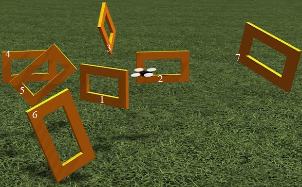
- 7 gates.
- The position and orientation of each gate are known.
Optimal Control Formulation
- Use
GPOPS-II.- An optimal control software.
- Can solve
multi-phase nonlinear optimal control problemsusing- sparse nonlinear programming
- hp-adaptive Gaussian quadrature collocation
Cost function
\[J = \rho \underbrace{t_f}_{\text{Term 1}} + \underbrace{\int_0^{t_f} \mathbf{u}^T(t) R_{uu}\mathbf{u}(t)dt}_{\text{Term 2}},\]where
Term 1: the final time.Term 2: the amount of control used.- \(\rho = 25\).
- \(R_{uu} = I\), identity matrix.
Phases
Specify constraints needs to be considered when the quadrotor is traversing each specific gate.
- Phases:
- 7 phases
- 1: begining to gate 1.
- \(\cdots\).
- pass through the center of each gate at the end of each phase.
- 7 phases
Constraints
Gate constraints:
- two constraints per gate
- pass through the center on each gate.
- force the velocity vector to be inside the cone of the gate center.
- \(\theta_{vel}\le \theta_{cone}\), where \(\theta_{cone} = 60^\circ\).
- prevent the quadrotor from simply passing through the center of the gate but not traversing it.
Field of view constraint:
- the camera of the quadrotor should be pointing to the gate in the traversing point.
- the constraints are imposed at the end of each phase.
where
- \(\psi\) is the yaw angle.
- \(\theta\) is the pitch angle.
- \(\delta_\theta = 30^\circ\).
Input constraints
\[T\in[0,20] N, \tau \in [-5,5] Nm.\]Gate state constraints
\[X\in[\min(X_{gate_i}, X_{gate_{i+1}}) - \delta_X, \max(X_{gate_i}, X_{gate_{i+1}}) + \delta_X],\]where \(\delta_X =0.5m\) acts as a margin.
Solving
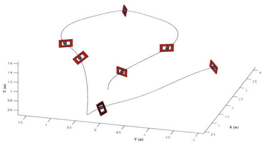
- Convergence time: 6m, 55s.
- Optimal cost was \(J^* = 295.22\).
- Final time was \(t_f = 4.278s\).
Limitations
- Assumed that the
environmentis completely known, which is unrealistic in many situations. - The computation time is
far from real-time.
Real-time Planning in Unknown Environments
Motivation
Real-time
- Use the full nonlinear dynamics of the quadrotor are not appropriate for
real-timeapplications. - To reduce the complexity of the optimization problem, use the
differential flatnessof the quadrotor. - Use a
simple integrator modelin the local planner to generate a trajectory. - Then, track it.
CTG
- Global planner does not account for the dynamics results in erratic behaviors when the environment model is changing repidly.
- Thus, a need of an accurate cost-to-go (CTG) calculation that captures both the global environment and the dynamic feasibility.
- Also, maintaining relatively low computation times at the same time.
Computational cost
- The choice of the
representation of the environmentandsize of the global maphave a significant impact on the computational cost. - Challenge:
- How to combine the global knowledge (slower rate) with the high-rate local information in the planner representation of the environment.
- How to
optimize the planning and mapping algorithms to achieve higher rates, suitable for aggressive flights.
Problem Formulation
Planning
- Computing a
dynamically feasible trajectoryfrom the start to the goal is typically intractable. Global plannergives the local planner a notion of CTG or traversability in certain directions.Local plannerdeviates around the nearby obstacles and chooses the terminal point accordingly.- Key to the
CTGcalculation is thetrade-off between accuracy and computation time. Jump Point Search (JPS)is used as aglobal plannerto find the shortest path from the current position to the goal.- JPS VS A\(^*\):
- JPS runs an order of magnitude faster.
- Still guarantee completeness and optimality.
- The only assumption is a uniform grid.
- JPS is only done for
position, reduce the computational burden.
Local plannermonitors the JPS solution for drastic changes between each replan.- If a large change is detected:
- A new path, composed of a high, medium, and low fidelity model is created for the current and last JPS solution.
- It is able to capture a subset of the dynamics while maintaining computational tractability.
- Multi-fidelity paths are compared and the path with lowest cost is selected for execution.
- Hierarchical trajectory consists of
- a jerk-controlled part
- a velocity-controlled part
- a geometric part
- If a large change is detected:
Quadrotor is modeled using triple integrator dynamics:
- State: \(x^T = [x^T\quad v^T \quad a^T]\).
- Control input: \(u = j\).
Convex optimization problem to find the trajectory:
\[\min_{u_{0:N-1}}\sum_{i=0}^{N-1}\Vert u_i\Vert^2 + (x_N-x_f)^T Q (x_N-x_f),\] \[\begin{aligned} s.t.\quad & x_0 = x_{init}, \\ & x_{k+1} = M_1 x_k + M_2 u_k, \forall k = 0:N-1, \\ & \Vert v_k\Vert_\infty \le v_{max}, \forall k = 1:N, \\ & \Vert a_k\Vert_\infty \le a_{max}, \forall k = 1:N, \\ & \Vert u_k\Vert_\infty \le j_{max}, \forall k = 0:N-1. \end{aligned}\]Where
- \(N\) is the number of discretization steps.
- \(dt\) is embedded in \(M_1,M_2\): \(dt = \max\{ T_{v_i}, T_{a_i}, T_{j_i} \}/N\).
- A lower bound on the time required per interval.
- Increase in each iteration until the problem converges.
Solver: CVXGEN.
Mapping
- A sliding map, moves with the quadrotor.
- represent the world.
- It tries to minimize the accumulated estimation error.
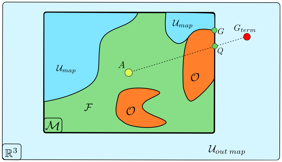
- The map contains:
- The map \(M\) contains:
- free-known space \(F\)
- Known obstacles \(O\)
- unknown space \(U_{map}\)
- Total unknown space: \(U = U_{map}\cup U_{out}\)
- \(Q\) is the projection into the map of the terminal goal \(G_{term}\) in the direction of \(\overrightarrow{AG_{term}}\).
- \(G\) is the closest free or unknown frontier point to \(Q\), which is selected as the goal.
- The map \(M\) contains:
Collision check:
- The jerk-controlled trajectory is considered collision-free if it does not intersect \(O\cup U\).
- The velocity-controlled primitive is forced to pass through the waypoints of the JPS solution.
- JPS path is guaranteed not to hit \(O\).
- JPS is an optimistic global planner, but the local planner is conservative.
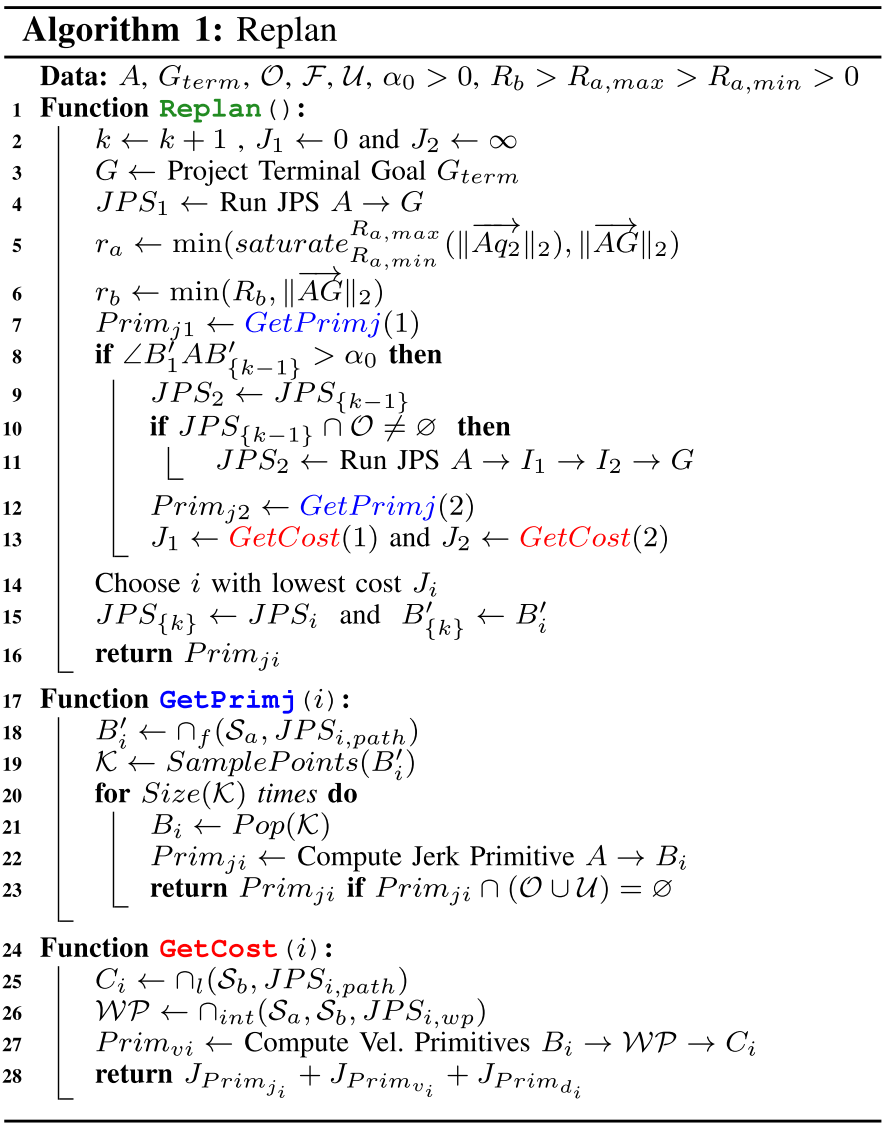
Algorithm
Planning
Notation:
- \(A\) is the state taken some steps ahead of the current position of the quadrotor.
- \(S_a,S_b\) are two concentric spheres with center in \(A\).
JPSdenotes the shortestpiece-wise linear pathfound by running JPS between \(A\) and \(G\).- Waypoints: \(JPS_{wp} = (q_1,q_2,\cdots,q_n)\).
- Path: \(JPS_{path} = (\overline{q_1q_2},\cdots,\overline{q_{n-1}q_n})\).
- \(B' = \cap_f(S_a,JPS_{path})\): the first intersection.
- \(C = \cap_l(S_b,JPS_{path})\): the last intersection.
- \(\cap(S_a,S_b,JPS_{wp})\) denotes all the elements of \(JPS_{wp}\) that are intermediate between \(B'\) and \(C\).
The whole trajectory planned is divided into three primitives:
\[Prim_j\cup Prim_v \cup Prim_d.\]- \(Prim_j\) is a jerk-controlled primitive that has \(A\) as initial state and a final stop condition in the point \(B\).
- \(B\): defined as the point in the sphere \(S_a\) near to \(B'\), and guarantees that \(Prim_j\cap(O\cup U) = \varnothing\).
- \(Prim_v\) is the composition of several velocity-controlled primitives between each pair of consecutive points of \((B,q_r,\cdots,q_{s-1},C)\).
- \(Prim_d\) is the part of JPS that goes from \(C\) to \(G\), \(Prim_d\cap O = \varnothing\).
Time-normalized costs:
\[\begin{aligned} J_{Prim_j} & = \frac{N\cdot dt}{j_{max}^2}\cdot \sum_{i=0}^{N-1}\Vert j_i\Vert_2^2, \\ J_{Prim_v} & = \sum_{k=0}^{s-r}\left( \frac{N\cdot dt_k}{v_{max}^2}\cdot \sum_{i=0}^{N-1}\Vert v_{k_i}\Vert_2^2 \right), \\ J_{Prim_d} & = \frac{\Vert q_s - C\Vert_2}{v_{max}} + \sum_{k=s}^{n-1}\left( \frac{\Vert q_{k+1} - q_k\Vert_2}{v_{max}} \right). \end{aligned}\]Total cost of the planned trajectory:
\[J = J_{Prim_j} + J_{Prim_v} + J_{Prim_d}.\]- Combine a high-fidelity model near the quadrotor.
- A medium-fidelity model in the medium part.
- Model without dynamics for the farthest part of the trajectory.
The cost is an approximation of the total cost of the jerk-controlled trajectory that goes from \(A\to G\),
- but it is much
faster to compute. - also, it is more accurate than relying only on jerk for the first part, and distance in the JPS path for the rest.
Algorithm:
Mapping and Planning Integration
- Fuse a
depth mapinto the occupancy grid using 3D Bresenham’s line algorithm for ray-tracing. - The mapper update rate is slower than the sensor frame rate.
- Address by storing the \(k\)-d trees of the point clouds that have arrived since the most recent map was published.
- Collision checks are then done using the occupancy grid and some of the saved \(k\)-d trees of the instantaneous point clouds.
- Ensure that the local planner relies both on
- the most recent fused map with global knowledge of the world.
- and up-to-date point clouds that contain the instantaneous sensing data.
Simulation
Set up
- C++ code for dynamics engine
- Gazebo to simulate perception data
- depth map
- FOV: \(90^\circ\).
- Range: \(10m\).
- point cloud
- depth map
Comparison
Methods:
- Incremental approach.
- Random goal.
- Optimistic RRT\(^*\)
- unknown space = free
- Conservative RRT\(^*\)
- unknown space = occupied
- Next-best-view planner (NBVP)
- Safe Local Exploration
Environment:
- random cluttered forest with an obstacle density of \(0.1 obstacles/m^2\).
- Sliding map size is \(20m\times 20m\).
- voxel size is \(10cm\).
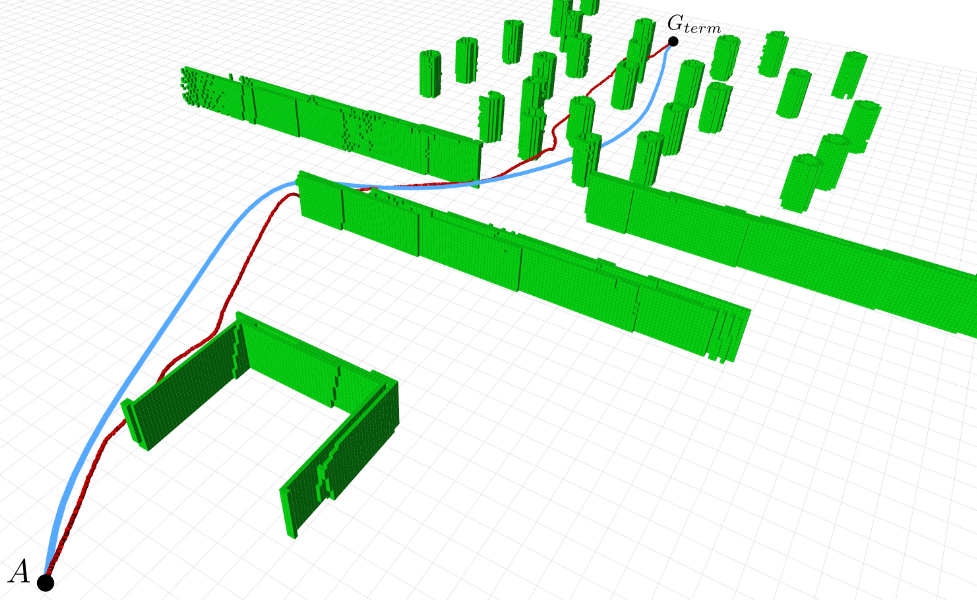
Blue (56.3m): the global optimal trajectory.- The map is completely known.
Red (56.8m): the trajectory generated by the planning algorithm.- The world is not known.
- Able to obtain a near-optimal path even when the world is discovered gradually.
Experiment
Quadrotor
- Qualcomm Snap Dragon Flight
- Nvidia Jetson TX2
- Intel RealSense Depth Camera D435
Procedure
- Perception
- Planning
- Control
All the procedure runs onboard.
Limitation
- Sometimes it can be quite
conservative.- Generate low-speed trajectories.
- Because of the final stop condition imposed inside \(F\).
Fast and Safe Trajectory Planner (FASTER)
Motivation
Navigating through unknown environments entails repeatedly generating collision-free, dynamically feasible trajectories.
Consider a sliding map \(M\): \(\mathbb{R}^3 = O\cup F \cup U = M\cup U\).
- \(F\): free-known
- \(O\): occupied-known
- \(U\): unknown space
- \(F\cup O \subset M\).
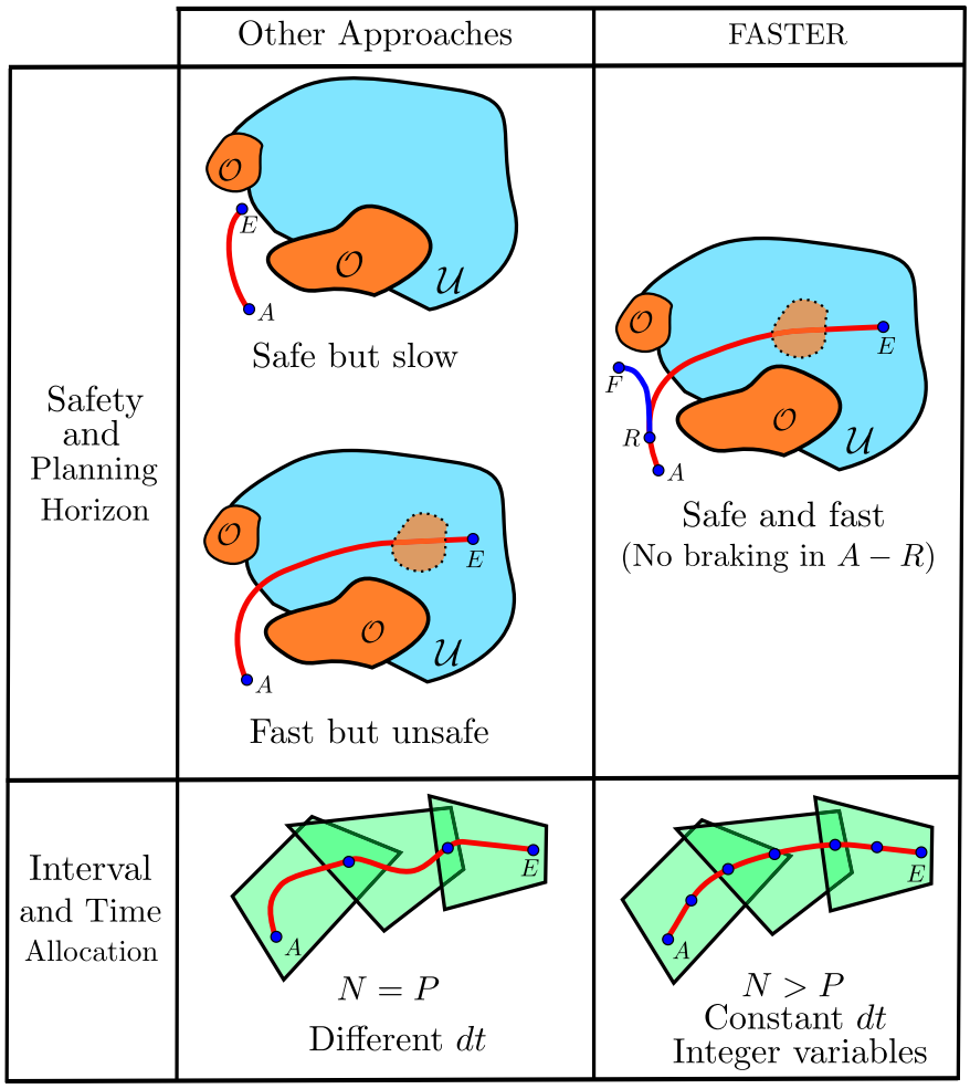
Safety is usually guaranteed by constructing trajectories that are entirely contained in \(F\) with a final stop condition.
- Generate motion primitives that do not intersect \(O\cup U\).
Problem:
- the above method leads to
slow trajectoriesin scenarios where \(F\) is small compared to \(O\cup U\).
Decomposing the free space into \(P\) overlapping polyhedra along a path connecting a start \(A\to E\).
- The usual approach is to divide the total trajectory into \(N = P\) intervals.
- This simplifies the problem because no integer variables are needed.
- Each interval is forced to be in one specific polyhedron.
- The time allocation problem becomes much harder.
- Trajectory ends up being much more conservative.
- because the optimizer is only allowed to move the extreme points of each interval of the trajectory in the overlapping areas.
Contributions
Present an optimization-based approach that
- reduce the aforementioned limitations by solving for
two optimal trajectoriesat every planning step.- one in \(U\cup F\)
- another one in \(F\)
- Use \(N > P\) intervals.
- Encoding the optimization problem as a MIQP.
- Propose an efficient way to compute a heuristic of \(dt\) using the result obtained in the previous replanning iteration.
Algorithm
Planning
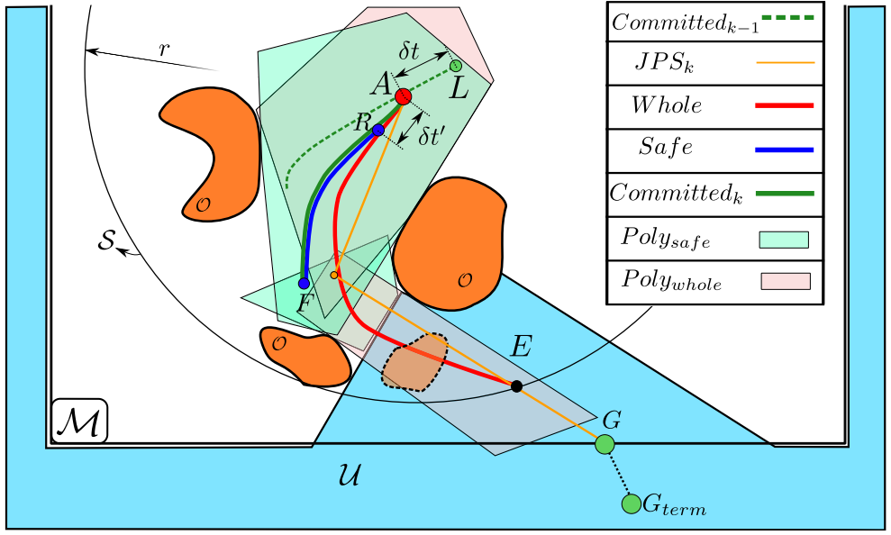
- JPS is used as a
global plannerto find the shortest piece-wise linear path between two points. - For
local planner, distinguish three different jerk-controlled trajectories:- Whole trajectory: goes from \(A\to E\), is contained in \(F\cup U\), it has a final stop condition.
- Safe trajectory: goes from \(R\to F\).
- \(R\) is a point in the whole trajectory.
- \(F\) is any point inside the polyhedra obtained by doing a convex decomposition of \(F\).
- It is completely contained in the free-known space \(F\).
- It has a final stop condition to guarantee safety.
- Committed trajectory: consists of two pieces:
- The interval \(A\to R\) of the whole trajectory.
- The safe trajectory.
- It is guaranteed to be inside \(F\).
- This trajectory is the one that the quadrotor will execute in the case:
- no feasible solutions are found in the next replanning steps.
The whole trajectory will be a spline consisting of third degree polynomials.
Matching the cubic form of the position for each interval as:
\[x_n(\tau) = a_n \tau^3 + b_n \tau^2 + c_n \tau + d_n, \tau\in[0,dt], n = 0:N-1.\]Using the expression of a cubic Bezier curve:
\[x_n(\tau) = \sum_{k=0}^3\begin{bmatrix} 3 \\ k \end{bmatrix}\left( 1 - \frac{\tau}{dt} \right)^{3-i}\left( \frac{\tau}{dt} \right)^i r_{nk},\tau\in[0,dt].\]Solve for the control points \(r_j(j = 0:3)\) associated with the curve:
\[\begin{aligned} r_{n0} & = d_n, \\ r_{n1} & = \frac{c_n dt + 3d_n}{3}, \\ r_{n2} & = \frac{b_n dt^2 + 2c_n dt + 3d_n}{3}, \\ r_{n3} & = a_n dt^3 + b_n dt^2 + c_n dt + d_n. \end{aligned}\]Denote the sequence of \(P\) overlapping polyhedra as:
\[\{ A_p \le c_p \}, p = 0:P-1.\]Introduce binary variables \(b_{np}\).
- \(P\) variables for each interval \(n = 0:N-1\).
The curve is contained in the convex hull of its control points, we can ensure that the whole trajectory will be inside this convex corridor by forcing that all the control points are in the same polyhedron:
- constraint \(b_{np} = 1\).
- At least in one polyhedron with the constraint \(\sum_{p = 0}^{P-1} b_{np}\ge 1\).
- The optimizer is free to choose in which polyhedron exactly.
The complete MIQP can be solved in each replanning step for both:
- safe trajectory
- whole trajectory
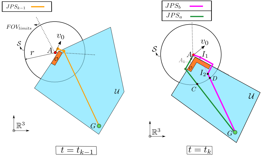
Let \(L\) be the current position of the quadrotor.
The point \(A\) is chosen in the committed trajectory of the previous replanning step with an offest \(\delta t\) from \(L\).
- \(\delta t\) is computed by multiplying the total time of the previous replanning step by \(\alpha\ge 1\).
- Dynamically change this offset to ensure that most of the times the
solvercan find the next solution in less than \(\delta t\).
The final goal \(G_{term}\) is projected into the sliding map \(M\) in the direction \(\overrightarrow{G_{term}A}\) to obtain the point \(G\).
Run JPS from \(A\to G\) to obtain \(JPS_a\).
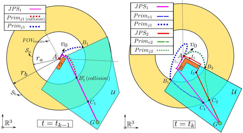
The local planner has to choose which direction of JPS solution should be used to guide the optimization.
- Take into account the
dynamics of the quadrotor. - Modify the \(JPS_{k-1}\) so that it does not collide with the new obstacles.
- Find the points \(I_1,I_2\).
- Run JPS three times.
- Then, modified as \(JPS_b\).
- Compute the a lower bound on \(dt\) for both \(A\to C\) and \(A\to D\).
- Find the
costassociated with each direction by adding this \(dt_a, dt_b\). - Find the
timeit would take to go \(C\to G\) following the JPS solution and flying at \(v_{max}\). - Finally, the one with
lowest costis chosen via \(JPS_k \gets \arg\min_{JPS_a,JPS_b}\{ J_a,J_b \}\).
The whole trajectory is obtained as follows:
- Do the convex decomposition of \(U\cup F\) around the part of \(JPS_k\) that is inside the sphere \(S\).
- This gives a series of overlapping polyhedra that we denote as \(Poly_{whole}\).
- Solve the MIQP using these polyhedral constraints to obtain the
whole trajectory.
The safe trajectory is obtained as follows:
- Choose the point \(R\) along the
whole trajectoryas the start of the safe path.- \(R\) should be chosen as far as possible from \(A\), so that
- \(\delta t\) can be chosen bigger in the next replanning step.
- still guarantee that \(A\) is not chosen on the safe path.
- The point \(R\) too close to \(H\) may lead to an infeasible problem for the safe trajectory optimizer.
- Choose \(R\) as the nearest state to \(H\), that is not in inevitable collision with \(U\).
- To compute an approximation of this state in a very efficient way, choose \(R\) as the last point that satisfies: \(sign[v_{R,j}(x_{H,j} - x_{R,j})]\frac{v_{R,j}^2}{2\vert a_{max}\vert} < \vert x_{H,j} - x_{R,j}\vert, j = \{x,y\}.\)
- Ignore the axis \(z\) in the computation to reduce the conservativeness of the heuristic.
- \(R\) should be chosen as far as possible from \(A\), so that
- Run convex decomposition in \(F\) using the part of \(JPS_{in}\) that is in \(F\).
- Obtain the polyhedra \(Poly_{safe}\).
- Solve the MIQP from \(R\) to any point \(F\) inside \(Poly_{safe}\).
- This point \(F\) is chosen by the optimizer.
In the convex decompositions above, one polyhedron is created for each segment of the piecewise linear paths, to obtain a less conservative solution, i.e. bigger polyhedra:
- Check the length of the segments of the JPS path.
- Creat more vertexes if this length exceeds certain threshold \(l_{max}\).
- Truncate the number of segments in the path to ensure that the number of polyhedra found dose not exceed a threshold \(P_{max}\).
The committed trajectory is obtained as follows:
- Concatenate the piece \(A\to R\) of the
whole trajectoryand thesafe trajectory.
FASTER Algorithm:
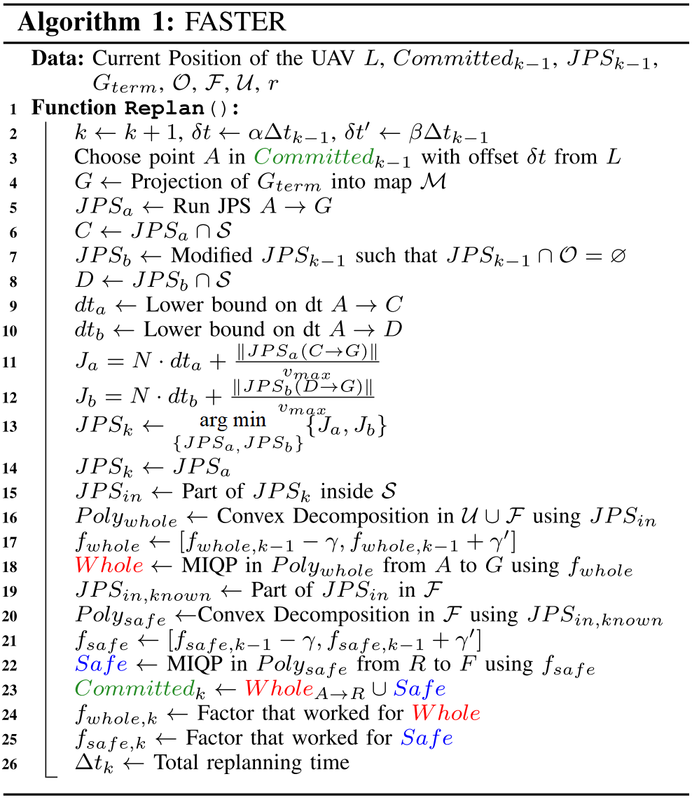
In the FASTER algorithm, we have run two decoupled optimization problems per replanning step:
- One for
whole trajectory. - One for
safe trajectory.
This ensures that the piece \(A\to R\) is not influenced by the breaking maneuver \(R\to F\). Therefore, guarantee a higher nominal speed on the first piece.
The intervals \(L\to A\) and \(A\to R\) have been designed so that, with high probability, at least one replanning step can be solved within that interval.
To prevent the cases where both \(A,R\) are in \(F\), but the piece \(A-R\) is not:
- check that piece \(A-R\) against collision with \(U\).
If any of the two optimizations fails, or the piece \(A-R\) intersects \(U\):
- the quadrotor
does not commit to any trajectory in that replanning step. - continues executing the
committed trajectoryof the previous replanning step.
Mapping
Use the same framework:
- A sliding map centered on the quadrotor that moves as the quadrotor flies.
- Fusing a
depth mapinto the occupancy grid using the3D Bresenham's line algorithmfor ray-tracing. - \(O,U\) are inflated by the radius of the quadrotor to ensure safety.
Simulation
- Test in 10 random forest environments.
- Compare the flight distances achieved against the six methods.
- Dynamic constraints:
- \(v_{max} = 5m/s\).
- \(a_{max} = 5m/s^2\).
- \(j_{max} = 8m/s^3\).
Experiment
- Quadrotor
- Perception: Intel RealSense D435
- Mapper and planner: Intel NUC
- Control: Qualcomm SnapDragon Flight
- IMU
Key properties of this planner
- leads to a higher nominal speed than the other algorithms by planning both in \(U,F\).
- Ensures safety by having always a safe path planned at the beginning of every replanning step.
Conclusion
- Assume a completely known world, and solving the full nonlinear optimal control problem with full nonlinear dynamics of the quadrotor.
- can not guarantee the real-time.
- Use the differential flatness of the quadrotor to use a simple triple integrator model as the dynamics of the quadrotor.
- Assume the world is not known.
- The planner was allowed to optimize in the free-known space \(F\).
- The flight speed is not fast, because of the final stop condition imposed inside \(F\).
- Planning both in free-known and unknown \(F\cup U\) space.
- Have a safe trajectory planned in \(F\).
- High-speed flights in completely unknown environments, up to \(7.8m/s\).
Future work
- Inclusion of
dynamic obstacles. - Apply
Tube-Based MPCto guarantee that the quadrotor is inside a tube around a nominal trajectory. - Integration the planning and mapping framework with a
state estimation algorithm(VIO), take into account the uncertainty in the state estimation to generate the trajectory.
References
- J. Tordesillas, “Trajectory Planner for Agile Flights in Unknown Environments,” 2019.