Implementation of CNN by Tensorflow
Tensorflow
Computation Graph
Tensorflow是基于graph的并行计算模型,Computation Graph 包括以下部分:
Placeholder: variables used in place of inputs to feed to the graphVariables: model variables that are going to be optimized to make the model perform betterModel (CNN layers): a mathematical function that calculates output based on placeholder and model variablesLoss Function: guide for optimization of the model variablesOptimizer: update method for tuning model variables
注:在定义graph时,没有进行任何数据的计算操作,只是建立nodes和symbols。
A simple example
用Tensorflow计算:\(a = (b+c)*(c+2)\).
变量定义
import tensorflow as tf
import numpy as np

print(tf.__version__)

const = tf.constant(2.0, name='const')
b = tf.Variable(2.0, name='b')
#b = tf.placeholder(tf.float32, [None, 1], name='b')
c = tf.Variable(1.0, dtype=tf.float32, name='c')
运算函数
d = tf.add(b, c, name='d')
e = tf.add(c, const, name='e')
a = tf.multiply(d, e, name='a')
变量初始化
Tensorflow中所有变量必须经过初始化才能使用。
init_op = tf.global_variables_initializer()
运行graph计算
运行graph需要调用tf.Session()函数创建一个会话,通过该会话与graph进行交互。
with tf.Session() as sess:
    sess.run(init_op)
    a_out = sess.run(a)
    #a_out = sess.run(a, feed_dict={b: np.arange(0, 10)[:, np.newaxis]})
    print('a is {}' .format(a_out))
Tensorflow placeholder
如果让变量b可以接收任意值,则需要Tensorflow调用占位符函数:
b = tf.placeholder(tf.float32, [None, 1], name='b')    # None表示不确定第一个维度的大小,对应tensor数量或样本数量

a_out = sess.run(a, feed_dict={b: np.arange(0, 10)[:, np.newaxis]})
Source Code
The source code is also available on Github.
import tensorflow as tf
import numpy as np

print(tf.__version__)

const = tf.constant(2.0, name='const')
#b = tf.Variable(2.0, name='b')
#b = tf.placeholder(tf.float32, [None, 1], name='b')
b = tf.placeholder(tf.float32, [None, ], name='b')
c = tf.Variable(1.0, dtype=tf.float32, name='c')

d = tf.add(b, c, name='d')
e = tf.add(c, const, name='e')
a = tf.multiply(d, e, name='a')

init_op = tf.global_variables_initializer()

with tf.Session() as sess:
    sess.run(init_op)
    # a_out = sess.run(a)
    #a_out = sess.run(a, feed_dict={b: np.arange(0, 10)[:, np.newaxis]})
    a_out = sess.run(a, feed_dict={b: np.arange(0, 10)})
    print('a is {}' .format(a_out))
Implement the NN by Tensorflow
加载数据集
import tensorflow as tf
from tensorflow.examples.tutorials.mnist import input_data

mnist = input_data.read_data_sets("MNIST_data/", one_hot=True)  # 对label进行one-hot编码,如:标签4表示为[0,0,0,0,1,0,0,0,0,0],与神经网络输出层的格式对应
变量定义
# hyperparameters
learning_rate = 0.5
epochs = 10
batch_size = 100

# placeholder
x = tf.placeholder(tf.float32, [None, 784]) # inputs image 28*28
y = tf.placeholder(tf.float32, [None, 10])  # labels 0-9的one-hot编码
NN参数定义
# hidden layer => w, b
w1 = tf.Variable(tf.random_normal([784, 300], stddev=0.03), name='w1')
b1 = tf.Variable(tf.random_normal([300]), name='b1')

# output layer => w, b
w2 = tf.Variable(tf.random_normal([300, 10], stddev=0.03), name='w2')
b2 = tf.Variable(tf.random_normal([10]), name='b2')
构造 hidden layer
\[z = x*w+b,\] \[h = relu(z).\]# hidden layer
hidden_out = tf.add(tf.matmul(x, w1), b1)
hidden_out = tf.nn.relu(hidden_out)
输出层输出预测值
# output predict value
y_ = tf.nn.softmax(tf.add(tf.matmul(hidden_out, w2), b2))
y_clipped = tf.clip_by_value(y_, 1e-10, 0.9999999)
定义 loss function
分类问题中常用Cross Entropy作为loss function:
\[L = - \frac{1}{m} \sum_{i=1}^m \sum_{j=1}^n y_j^i \log y_{j\_}^i + (1 - y_j^i) \log (1 - y_{j\_}^i).\]其中,\(n\)表示标签数,\(m\)表示样本数。
# loss function
cross_entropy = -tf.reduce_mean(tf.reduce_sum(y*tf.log(y_clipped) + (1-y) * tf.log(1-y_clipped), axis=1))
Optimizer优化方法定义
optimizer = tf.train.GradientDescentOptimizer(learning_rate = learning_rate).minimize(cross_entropy)
minimize(cross_entropy) does two things:
- Computes the gradient of the loss function w.r.t. all the variables (\(w\) and \(b\)).
- Applies the gradient updates to all those variables.
定义精确度分析
# accuracy analysis
correct_prediction = tf.equal(tf.argmax(y, 1), tf.argmax(y_, 1))
accuracy = tf.reduce_mean(tf.cast(correct_prediction, tf.float32))
初始化变量
# init variables
init_op = tf.global_variables_initializer()
运行graph计算
# begin the session
with tf.Session() as sess:
sess.run(init_op) # init the variables
total_batch = int(len(mnist.train.labels) / batch_size)
for epoch in range(epochs):
avg_cost = 0
for i in range(total_batch):
batch_x, batch_y = mnist.train.next_batch(batch_size = batch_size)
_, c = sess.run([optimizer, cross_entropy], feed_dict={x: batch_x, y:batch_y})
avg_cost += c / total_batch
print('Epoch:', (epoch+1), 'cost = {:.3f}' .format(avg_cost))
print('Accuracy:', sess.run(accuracy, feed_dict={x: mnist.test.images, y: mnist.test.labels}))
输出结果
Epoch: 1 cost = 0.608
Epoch: 2 cost = 0.229
Epoch: 3 cost = 0.169
Epoch: 4 cost = 0.134
Epoch: 5 cost = 0.108
Epoch: 6 cost = 0.089
Epoch: 7 cost = 0.077
Epoch: 8 cost = 0.062
Epoch: 9 cost = 0.055
Epoch: 10 cost = 0.049
Accuracy: 0.9761
TensorBoard
We can visualize the computation graph and monitor the scalars like loss, accuracy and parameters like weights and biases.
Creating FileWriter
To enable this visualization, we first create a FileWriter object. As TensorBoard essentially visualizes the training logs, we need to store them before we can use TensorBoard.
# store the logs to ./graphs directory
writer = tf.summary.FileWriter('./graphs', graph=tf.get_default_graph())
Logging Dynamic Values
In order to log loss, accuracy and parameters, we need to create Summary nodes that can be executed inside a session.
# add summary
tf.summary.scalar("loss", cross_entropy)
tf.summary.scalar("accuracy", accuracy)
tf.summary.histogram("w1", w1)
tf.summary.histogram("b1", b1)
tf.summary.histogram("w2", w2)
tf.summary.histogram("b2", b2)
Merging Summary Operations
Merge these summary operations so that they can be executed as a single operation inside the session.
summary_op = tf.summary.merge_all()
Running and Logging the Summary operation
Now, we can run the Summary operation inside the session, and write its output to the FileWriter.
Note that epoch is the iteration index inside the training loop.
summary = sess.run(summary_op, feed_dict={x: batch_x, y:batch_y})
writer.add_summary(summary, epoch)
Open the TensorBoard
tensorboard --logdir=/path/to/log-directory
Then, open the website which obtained in the terminal, such as: http://UAV:6006. The variety of the variables display as follows.

- Accuracy

- Loss
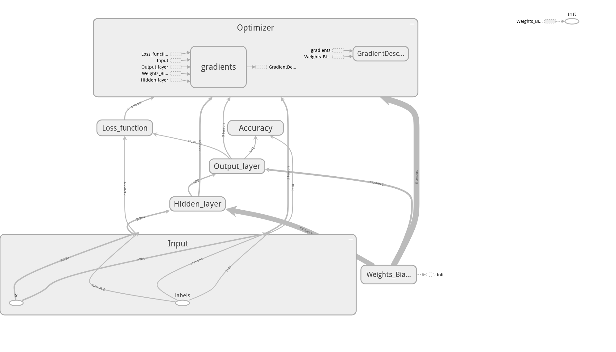
Making the Graph Readable
By default the graphs look very messy. We can clean them up by adding a name scope to the nodes.
with tf.name_scope('Input'):
# placeholder
x = tf.placeholder(tf.float32, [None, 784], name="x") # input image 28*28
y = tf.placeholder(tf.float32, [None, 10], name="labels") # labels 0-9的one-hot编码
Source Code
The source code is also available on Github.
import tensorflow as tf
from tensorflow.examples.tutorials.mnist import input_data
mnist = input_data.read_data_sets("MNIST_data/", one_hot=True) # 对label进行one-hot编码,如:标签4表示为[0,0,0,0,1,0,0,0,0,0],与神经网络输出层的格式对应
# hyperparameters
learning_rate = 0.5
epochs = 100
batch_size = 100
with tf.name_scope('Input'):
# placeholder
x = tf.placeholder(tf.float32, [None, 784], name="x") # input image 28*28
y = tf.placeholder(tf.float32, [None, 10], name="labels") # labels 0-9的one-hot编码
with tf.name_scope('Weights_Biases'):
# hidden layer => w, b
w1 = tf.Variable(tf.random_normal([784, 300], stddev=0.03), name='w1')
b1 = tf.Variable(tf.random_normal([300]), name='b1')
# output layer => w, b
w2 = tf.Variable(tf.random_normal([300, 10], stddev=0.03), name='w2')
b2 = tf.Variable(tf.random_normal([10]), name='b2')
with tf.name_scope('Hidden_layer'):
# hidden layer
hidden_out = tf.add(tf.matmul(x, w1), b1)
hidden_out = tf.nn.relu(hidden_out)
with tf.name_scope('Output_layer'):
# output predict value
y_ = tf.nn.softmax(tf.add(tf.matmul(hidden_out, w2), b2))
y_clipped = tf.clip_by_value(y_, 1e-10, 0.9999999)
with tf.name_scope('Loss_function'):
# loss function
cross_entropy = -tf.reduce_mean(tf.reduce_sum(y*tf.log(y_clipped) + (1-y) * tf.log(1-y_clipped), axis=1))
with tf.name_scope('Optimizer'):
optimizer = tf.train.GradientDescentOptimizer(learning_rate = learning_rate).minimize(cross_entropy)
with tf.name_scope('Accuracy'):
# accuracy analysis
correct_prediction = tf.equal(tf.argmax(y, 1), tf.argmax(y_, 1))
accuracy = tf.reduce_mean(tf.cast(correct_prediction, tf.float32))
# init variables
init_op = tf.global_variables_initializer()
# add summary
tf.summary.scalar("loss", cross_entropy)
tf.summary.scalar("accuracy", accuracy)
tf.summary.histogram("w1", w1)
tf.summary.histogram("b1", b1)
tf.summary.histogram("w2", w2)
tf.summary.histogram("b2", b2)
summary_op = tf.summary.merge_all()
# begin the session
with tf.Session() as sess:
writer = tf.summary.FileWriter('./graphs', graph=tf.get_default_graph())
sess.run(init_op) # init the variables
total_batch = int(len(mnist.train.labels) / batch_size)
for epoch in range(epochs):
for i in range(total_batch):
batch_x, batch_y = mnist.train.next_batch(batch_size = batch_size)
sess.run(optimizer, feed_dict={x: batch_x, y:batch_y})
summary = sess.run(summary_op, feed_dict={x: batch_x, y:batch_y})
writer.add_summary(summary, epoch)
loss = sess.run(cross_entropy, feed_dict={x: batch_x, y:batch_y})
print('Epoch:', (epoch+1), 'loss = {:.3f}' .format(loss))
print('Accuracy:', sess.run(accuracy, feed_dict={x: mnist.test.images, y: mnist.test.labels}))
Implement the CNN by Tensorflow
Load the Dataset
import tensorflow as tf
from tensorflow.examples.tutorials.mnist import input_data

mnist = input_data.read_data_sets("./tensorflow_examples/MNIST_data/", one_hot=True)  # 对label进行one-hot编码,如:标签4表示为[0,0,0,0,1,0,0,0,0,0],与神经网络输出层的格式对应
Parameters Definition
# hyperparameters
learning_rate = 0.01
episodes = 2000
batch_size = 100

# Network parameters
num_input = 784
num_classes = 10
dropout = 0.75

# input placeholder
x = tf.placeholder(tf.float32, [None, num_input], name="x")
y = tf.placeholder(tf.float32, [None, num_classes], name="labels")

# dropout placeholder
keep_prob = tf.placeholder(tf.float32)
CNN Parameters
# layers weights and biases
weights = {
    # 5x5 conv, 1 input, 32 outputs
    'wc1': tf.Variable(tf.random_normal([5,5,1,32])),
    # 5x5 conv, 32 inputs, 64 outputs
    'wc2': tf.Variable(tf.random_normal([5,5,32,64])),
    # fully connected, 7*7*64 inputs, 1024 outputs
    'wf1': tf.Variable(tf.random_normal([7*7*64, 1024])),
    # output layer, 1024 inputs, 10 outputs
    'out': tf.Variable(tf.random_normal([1024, num_classes]))
}

biases = {
    'bc1': tf.Variable(tf.random_normal([32])),
    'bc2': tf.Variable(tf.random_normal([64])),
    'bf1': tf.Variable(tf.random_normal([1024])),
    'out': tf.Variable(tf.random_normal([num_classes]))
}
CNN Layers
# create some wrappers for simplicity
def conv2d(x, w, b, strides=1):
    x = tf.nn.conv2d(x, w, strides=[1, strides, strides, 1], padding='SAME')    # output:[batch_size, H, W, filter_num]
    x = tf.nn.bias_add(x, b)
    return tf.nn.relu(x)

def maxpool2d(x, k=2):
    return tf.nn.max_pool(x, ksize=[1, k, k, 1], strides=[1, k, k, 1], padding='SAME')

# CNN model
def conv_net(x, weights, biases, dropout):
    # reshape the input 784 features to match picture format [height*width*channel]
    # Tensor input become 4-D: [batch_size, height, width, channel]
    x = tf.reshape(x, shape=[-1, 28, 28, 1])

    # conv layer1
    conv1 = conv2d(x, weights['wc1'], biases['bc1'])    # [100,28,28,32]
    # maxpool layer1
    conv1 = maxpool2d(conv1)    # [100,14,14,32]

    # conv layer2
    conv2 = conv2d(conv1, weights['wc2'], biases['bc2'])    # [100,14,14,64]
    # maxpool layer2
    conv2 = maxpool2d(conv2)    # [100,7,7,64]

    # fully connected layer
    fc1 = tf.reshape(conv2, [-1, weights['wf1'].get_shape().as_list()[0]])  # [100,7*7*64]
    fc1 = tf.add(tf.matmul(fc1, weights['wf1']), biases['bf1']) # [100,1024]
    fc1 = tf.nn.relu(fc1)   # [100,1024]

    # dropput
    fc1 = tf.nn.dropout(fc1, dropout)   # [100,1024]

    # output
    out = tf.add(tf.matmul(fc1, weights['out']), biases['out']) # [100,10]

    return out  # [100,10]

# construct CNN model
logits = conv_net(x, weights, biases, keep_prob)
y_ = tf.nn.softmax(logits)
Loss Function
# loss function
loss = tf.reduce_mean(tf.nn.softmax_cross_entropy_with_logits(logits = logits, labels = y))
Optimizer
# optimizer
optimizer = tf.train.AdamOptimizer(learning_rate).minimize(loss)
Accuracy
# evaluate model
correct_pred = tf.equal(tf.argmax(y_, 1), tf.argmax(y, 1))
accuracy = tf.reduce_mean(tf.cast(correct_pred, tf.float32))
Initial Variables
# init variables
init_op = tf.global_variables_initializer()
TensorBoard
# tensorboard
tf.summary.scalar("loss", loss)
tf.summary.scalar("accuracy", accuracy)
tf.summary.histogram("wc1", weights['wc1'])
tf.summary.histogram("wc2", weights['wc2'])
tf.summary.histogram("wf1", weights['wf1'])
tf.summary.histogram("w_out", weights['out'])
tf.summary.histogram("bc1", biases['bc1'])
tf.summary.histogram("bc2", biases['bc2'])
tf.summary.histogram("bf1", biases['bf1'])
tf.summary.histogram("b_out", biases['out'])
summary_op = tf.summary.merge_all()
Run Session
with tf.Session() as sess:
    sess.run(init_op)
    writer = tf.summary.FileWriter('./tensorflow_examples/multi_layer_CNN_graphs', graph=tf.get_default_graph())

    # total_batch = int(len(mnist.train.labels) / batch_size)

    for episode in range(episodes):
        # for i in range(total_batch):
        batch_x, batch_y = mnist.train.next_batch(batch_size)
        sess.run(optimizer, feed_dict={x: batch_x, y: batch_y, keep_prob: dropout})

        loss_value = sess.run(loss, feed_dict={x: batch_x, y: batch_y, keep_prob: dropout})
        print('Episode: {}, loss: {}' .format(episode+1, loss_value))

        summary = sess.run(summary_op, feed_dict={x: batch_x, y: batch_y, keep_prob: dropout})
        writer.add_summary(summary, episode)

    print('Accuracy:', sess.run(accuracy, feed_dict={x: mnist.test.images, y: mnist.test.labels, keep_prob: dropout}))
Source Code
The source code is available on Github.