Wasserstein Robust Reinforcement Learning
Motivation
Although significant progress has been made on developing algorithms for learning large-scale and high-dimensional reinforcement learning tasks, these algorithms often over-fit to training environments and fail to generalise across even slight variations of transitions dynamics.
Robustness to changes in transition dynamics is a crucial component for adaptive and safe RL in real-world environments.
Contributions
- Propose a robust RL algorithm that can cope with both discrete and continuous state and action spaces with significant robust performance on low and high-dimensional control tasks.
- The algorithm is in the “RL setting”, not the “MDP setting” where the transition probability matrix is known a priori. Put another way, although a simulator with parameterisable dynamics are required, the actual reference dynamics \(P_0\) need not be known explicitly nor learnt by the algorithm. The algorithm is
not model-basedin the traditional sense of learning a model to perform planning. - Dynamics uncertainty sets defined by Wasserstein distance.
Wasserstein Distance
The detailed description of Wassertein distance is here.
Algorithm
Robust Objectives and Constraints
Define the loss function as an algorithm that learns best-case policies under worst-case transitions:
\[\max_\theta \left[ \min_\phi \mathbb{E}_{\tau \sim p_\theta^\phi(\tau)}[R_{total}(\tau)] \right],\]where \(p_\theta^\phi(\tau)\) is a trajectory density function parameterised by both policies and transition models, \(\theta\) and \(\phi\), respectively.
Define the constraint set as follows:
\[W_\epsilon(P_\phi(\cdot), P_0(\cdot)) = \left\{ P_\phi(\cdot):W_2^2(P_\phi(\cdot \vert s,a), P_0(\cdot \vert s,a)) \le \epsilon, \quad \forall(s,a) \in S \times A \right\},\]where \(\epsilon \in \mathbb{R}_+\) is a hyperparameter used to specify the “degree of robustness”.
To remedy the problem that infinite number of constraints when considering continuous state and actions spaces, consider the average Wasserstein constraints instead:
\[\begin{aligned} \hat{W}_\epsilon^{average}(P_\phi(\cdot), P_0(\cdot)) & = \left\{ P_\phi(\cdot): \int_{(s,a)} P(s,a) W_2^2 (P_\phi(\cdot \vert s,a), P_0(\cdot \vert s,a)) d(s,a) \le \epsilon \right\} \\ & = \left \{ P_\phi(\cdot): \mathbb{E}_{(s,a) \sim P}\left[ W_2^2(P_\phi(\cdot \vert s,a), P_0(\cdot \vert s,a)) \right] \le \epsilon \right\}. \end{aligned}\]In above equation, the state-action pairs sampled according to \(P(s,a)\):
\[P(s \in S, a \in A) = P(a \in A \vert s \in S) P(s \in S) = \pi(a \in A \vert s \in S) \rho_\pi^{\phi_0}(s \in S).\]Then, Wasserstein robust RL objective:
Solution
The solution methodology follows an alternating procedure interchangeably updating one variable given the other fixed.
Updating Policy Parameters
The Wasserstein distance constraint is independent from policy parameters \(\theta\). Given a fixed set of model parameters \(\phi\), \(\theta\) can be updated by solving:
\[\max_\theta \mathbb{E}_{\tau \sim p_\theta^\phi(\tau)} [R_{total}(\tau)].\]Updating Model Parameters
Approximate the Wasserstein constraint by Taylor expansion up to second order:
\[W(\phi):=\mathbb{E}_{(s,a) \sim \pi(\cdot)\rho_\pi^{\phi_0}(\cdot)}\left[ W_2^2(P_\phi(\cdot \vert s,a), P_0(\cdot \vert s,a)) \right].\] \[\begin{aligned} W(\phi) & \approx W(\phi_0) + \nabla_\phi W(\phi_0)^T(\phi-\phi_0) + \frac{1}{2}(\phi-\phi_0)^T \nabla_\phi^2 W(\phi_0)(\phi-\phi_0) \\ & \approx \frac{1}{2}(\phi-\phi_0)^T \nabla_\phi^2 W(\phi_0)(\phi-\phi_0), \end{aligned}\]where \(W(\phi_0) = 0\), \(\nabla_\phi W(\phi_0) = 0\).
Then, update the model parameters given fixed policies:
\[\min_\phi \mathbb{E}_{\tau \sim p_\theta^\phi(\tau)} [R_{total}(\tau)] \quad s.t. \quad \frac{1}{2} (\phi - \phi_0)^T \mathbf{H}_0 (\phi - \phi_0) \le \epsilon,\]where \(\mathbf{H}_0\) is the Hessian of the expected squared 2-Wasserstein distance evaluated at \(\phi_0\):
\[\mathbf{H}_0 = \nabla_\phi^2 \mathbb{E}_{(s,a) \sim \pi(\cdot) \rho_\pi^{\phi_0}(\cdot)} \left[ W_2^2(P_\phi(\cdot \vert s,a), P_0(\cdot \vert s,a)) \right] \Big\vert_{\phi = \phi_0}.\]Approximate the loss function with first-order expansion, just like TRPO algorithm, then:
Thus,
\[\phi^{[j+1]} = \phi_0 - \sqrt{\frac{2\epsilon}{g^{[k,j]T}\mathbf{H}_0^{-1}g^{[k,j]}}} \mathbf{H}_0^{-1} g^{[k,j]},\]where \(g^{[k,j]}\) denotes the gradient evaluated at \(\theta^{[k]}\) and \(\phi^{[j]}\):
\[g^{[k,j]} = \nabla_\phi \mathbb{E}_{\tau \sim p_\theta^\phi (\tau)} [R_{total}(\tau)] \Big\vert_{\theta^{[k]}, \phi^{[j]}}.\]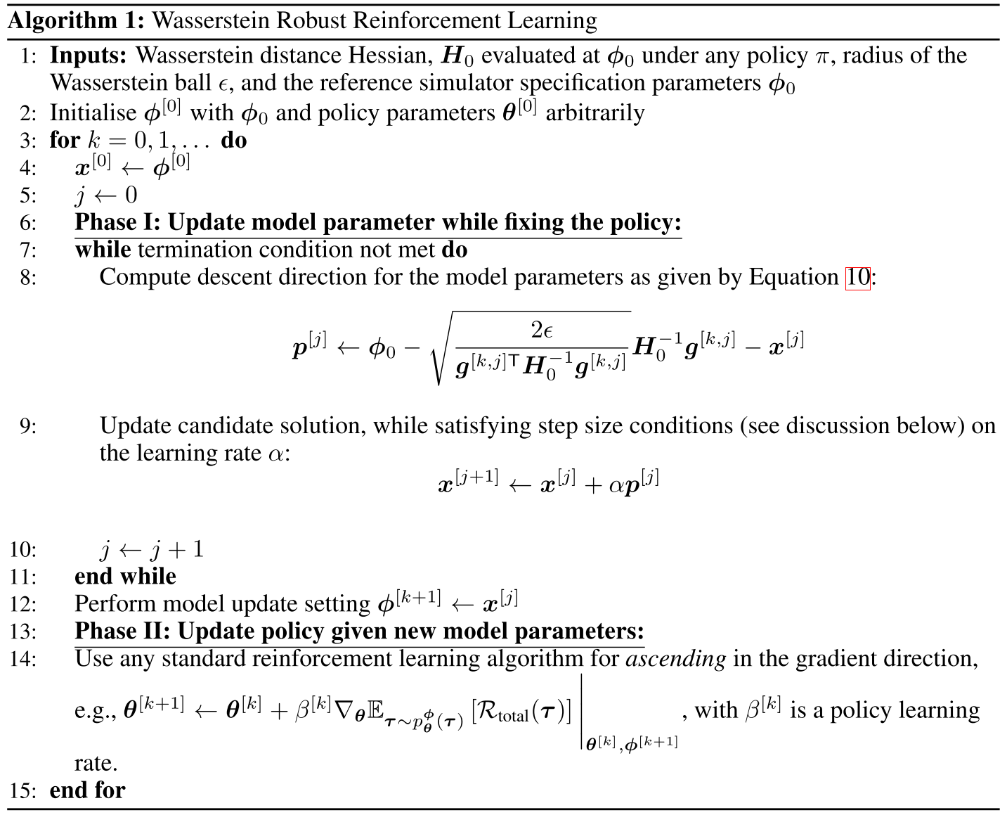
- Algorithm of Wasserstein Robust RL
Zero’th Order Algorithm Solver
A novel zero-order method is proposed for estimating gradients and Hessians to solve the algorithm on high-dimensional robotic environments.
Gradient Estimation
\[g = \nabla_\phi \mathbb{E}_{\tau \sim p_\theta^\phi (\tau)}[R_{total}(\tau)] = \frac{1}{\sigma^2}\mathbb{E}_{\xi \sim N(0, \sigma^2 I)} \left[ \xi \int_\tau p_\theta^{\phi+\xi}(\tau) R_{total}(\tau)d \tau \right].\]Proof:
Define the expected return with fixed policy parameters \(\theta\) as follows:
\[J_\theta(\phi) = \mathbb{E}_{\tau \sim p_\theta^\phi}[R_{total}(\tau)].\]Then, the Taylor expansion of \(J_\theta(\phi)\) with perturbation vector \(\xi \sim N(0, \sigma^2 I)\) can be obtained:
\[J_\theta(\phi+\xi) = J_\theta(\phi) + \xi^T \nabla_\phi J_\theta (\phi) + \frac{1}{2}\xi^T \nabla_\phi^2 J_\theta(\phi)\xi.\]Multiplying by \(\xi\), and taking the expectation on both sides of the obove equation:
\[\mathbb{E}_{\xi \sim N(0, \sigma^2 I)}[\xi J_\theta(\phi+\xi)] = \mathbb{E}_{\xi \sim N(0, \sigma^2 I)} \left[ \xi J_\theta(\phi) + \xi \xi^T \nabla_\phi J_\theta(\phi) + \frac{1}{2}\xi\xi^T \nabla_\phi^2 J_\theta(\phi)\xi \right] = \sigma^2 \nabla_\phi J_\theta(\phi).\]Then,
\[\nabla_\phi J_\theta(\phi) = \frac{1}{\sigma^2} \mathbb{E}_{\xi \sim N(0, \sigma^2 I)}[\xi J_\theta(\phi+\xi)].\]