Robust and Efficient Quadrotor Trajectory Generation for Fast Autonomous Flight
Motivation
- UAV Applications:
- Industrial inspection.
- Search and rescue.
- Package delivery.
- To achieve full autonomy in these scenarios, the
motion planningmodule plays an essential role in generating safe and smooth motions. - Two critical unsolved issues:
- No existing works guarantee to
generate safe and kinodynamic feasible trajectoryat a high success rate withlimited time and onboard computing resources.- Efficiency and robustness of the trajectory generation are essential.
- When a quadrotor flying at high speed in unknown environments, trajectories should be
re-generated constantlyin a very short time to avoid emergent threats.
- To ensure the kinodynamic feasibility of the generated motions, constraints on the velocity and acceleration are often enforced
conservatively.- As a result, the
aggressivenessof the generated trajectories are often hard to be tuned to satisfy applications where a high flight speed is preferable.
- As a result, the
- No existing works guarantee to
- Related work:
- Hard-Constrained methods:
- Minimum-snap trajectory generation.
- Represented as piecewise polynomials.
- Generated by solving a quadratic programming (QP) problem.
- One
common drawbackof the methods is that the time allocation of the trajectory is given by naive heuristics.- Significantly reduce the quality of the trajectory.
- Feasible solution can only be obtained by iteratively adding more constraints and solving the QP problem.
- It is
undesirable for real-time application.
- It is
- Ensure global optimality by the convex formulation, but distance to obstacles in the free space is ignored, which often results in
trajectories being close to obstacles. - Also, the kinodynamic constraints are conservative, making the trajectory’s
speed deficient for fast flight.
- Minimum-snap trajectory generation.
- Soft-Constrained methods:
- Formulate trajectory generation as a
non-linear optimization problem. - Take
smoothness and safetyinto account. - Methods:
- Generate
discrete-timetrajectories byminimizing its smoothness and collision costusing gradient descent methods. - Also, optimization can be solved by a
gradient-free sampling method. Continuous-timepolynomial trajectories method is presented to avoid numeric differentiation errors and is more accurate to represent the motions of drones.- But it suffers from a
low success rate.
- But it suffers from a
- To increase the success rate, a collision-free initial path firstly using an informed sampling-based path searching method.
- This path serves as a higher quality initial guess of non-linear optimization and thus improve the success rate.
- Trajectory is parameterized as a
uniform B-spline.- B-spline is
continuousby nature, which reduce the number of constraints. - It is also particularly useful for
local replanningthanks to its property of locality.
- B-spline is
- Generate
- These methods utilize gradient information to push trajectory far from obstacles.
- But, suffer from
local minimaand havingno strong guarantee of success rate and kinodynamic feasibility.
- Formulate trajectory generation as a
- Hard-Constrained methods:
Contributions
- Propose a robust and efficient quadrotor
motion planningsystem for fast flight in 3D complex environment.- Present a complete and robust online trajectory generation method.
- Adopt a kinodynamic path searching method to find a
safe,kinodynamic feasible, andminimum-time initialtrajectory in the discretized control space.- Linear quadratic minimum-time control is adopted.
- The initial path is refined in a carefully designed B-spline optimization.
- Improve the
smoothness and clearanceof the trajectory by aB-spline optimization, which incorporatesgradient informationfrom a Euclidean distance field and dynamic constraints efficiently utilizing the convex hull property of B-spline.- Unlike previous methods in which computational expensive line integrals along the trajectory are calculated.
- Redesigned to be simpler based on the convex hull property of B-Spline.
Improve the computation efficiency and convergent rate.
- An iterative time adjustment method is adopted to guarantee
dynamically feasibleandnon-conservativetrajectories.- Squeeze infeasible velocity and acceleration out from the profiles while avoiding constraining them conservatively.
- Code.
- ROS package.
- Video.
- Compare to existing works:
- Generate high-quality trajectories in cluttered environments in a
much shorter timewith ahigher success rate. - It can generate
aggressivemotion under the premise of dynamic feasibility.
- Generate high-quality trajectories in cluttered environments in a
Method
Kinodynamic path searching
- Front-end kinodynamic path searching module:
- Originated from the hybrid-state A* search1.
- Search for a safe and kinodynamic feasible trajectory that is minimal w.r.t.
time durationandcontrol costin a voxel grid map. - Searching loop is similar to the standard A* algorithm.
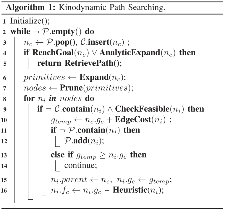
- \(P\) and \(C\) refer to the open and closed set.
- Instead of straight lines,
motion primitivesrespecting the quadrotor dynamic are used as graph edge. - A structure
Nodeis used to record a primitive.
Primitives Generation
- Motion primitives used in
Expand()function.
The differential flatness of quadrotor systems allows us to represent the trajectory by three independent 1D time-parameterized polynomial functions:
\[\mathbf{p}(t) := [p_x(t), p_y(t), p_z(t)]^T,\] \[p_\mu(t) = \sum_{k=0}^K a_k t^k,\]where \(\mu \in \{ x,y,z \}\).
Consider the quadrotor as a linear time-invariant (LTI) system.
State vector:
\[\mathbf{x}(t) := [\mathbf{p}(t)^T, \dot{\mathbf{p}}(t)^T, \cdots, \mathbf{p}^{(n-1)}(t)^T]^T \in X \subset \mathbb{R}^{3n}.\]Control input:
\[\mathbf{u}(t) := \mathbf{p}^{(n)}(t) \in U:=[-u_{max}, u_{max}]^3 \subset \mathbb{R}^3.\]Then, the state space model can be defined as:
\[\dot{\mathbf{x}} = \mathbf{A}\mathbf{x} + \mathbf{B}\mathbf{u},\] \[\mathbf{A} = \begin{bmatrix} 0 & I_3 & 0 & \cdots & 0 \\ 0 & 0 & I_3 & \cdots & 0 \\ \vdots & \vdots & \vdots & \ddots & \vdots \\ 0 & \cdots & \cdots & 0 & I_3 \\ 0 & \cdots & \cdots & 0 & 0 \end{bmatrix}, \quad \mathbf{B} = \begin{bmatrix} 0 \\ 0 \\ \vdots \\ 0 \\ I_3 \end{bmatrix}.\]The complete solution for the state equation is expressed as:
\[\mathbf{x}(t) = e^{\mathbf{A}(t)}\mathbf{x}(0) + \int_0^t e^{\mathbf{A}(t - \tau)} \mathbf{B}\mathbf{u}(\tau)d\tau.\]Then, the trajectory of the quadrotor can be obtained via the initial state \(\mathbf{x}(0)\) and the control input \(\mathbf{u}(t)\).
In Expand():
- Given the current state of the quadrotor.
- A set of discretized control inputs \(U_D \subset U\) is applied for duration \(\tau\).
- In practice, select \(n = 2\), corresponds to a double integrator.
- Each axis \([-u_{max}, u_{max}]\) is discretized uniformly as \(\left\{ -u_{max}, -\frac{r-1}{r}u_{max}, \cdots, \frac{r-1}{r}u_{max}, u_{max} \right\}\).
- Thus, results in \((2r+1)^3\) primitives.
Actual Cost and Heuristic Cost
Define the cost (time and control cost) of a trajectory as:
\[J(T) = \int_0^T \Vert \mathbf{u}(t)\Vert^2 dt + \rho T.\]Then, EdgeCost() calculates the cost of:
- a motion primitive generated with the discretized input \(\mathbf{u}(t) = \mathbf{u}_d\).
- and duration \(\tau\) as \(e_c = (\Vert \mathbf{u}_d \Vert^2 + \rho)\tau\).
Actual cost (start \(\to\) current):
- Use \(g_c\) to represent the
actual costof an optimal path from thestart state\(\mathbf{x}_s\) to thecurrent state\(\mathbf{x}_c\). - Let the optimal path consists of \(J\) primitives, then:
Heuristic cost (current \(\to\) goal):
- An admissible and informative
heuristicis essential tospeed up the searchingas in A*. Heuristic():- Minimize \(J(T)\) from \(\mathbf{x}_c\) to the goal state \(\mathbf{x}_g\) via Pontryagin’s minimum principle:
where \(p_{\mu c}, v_{\mu c}, p_{\mu g}, v_{\mu g}\) are the current and goal position and velocity.
To find the optimal time \(T\) that minimize the cost:
- Substitute \(\alpha_\mu, \beta_\mu\) into \(J^*(T)\).
- Find the roots of \(\frac{\partial J^*(T)}{\partial T} = 0\).
- Feasible trajectory is selected and denoted as \(T_h\).
- Heuristic cost denotes as \(h_c = J^*(T_h)\).
Then,
\[f_c = g_c + h_c = g_c + J^*(T_h).\]Analytic Expansion
- Due to the
discretized control input, it is difficult to have a primitive end exactly in the goal state. - Induce an analytic expansion scheme to
compensate for itand also tospeed up the searching.
AnalyticExpand():
- When a node is popped from the open set,
- if it passes the safety and dynamic feasibility check, the searching is terminated in advance.
The strategy is effective for improving efficiency especially in sparse environments, since
- it has a higher success rate,
- and terminates the searching earlier.
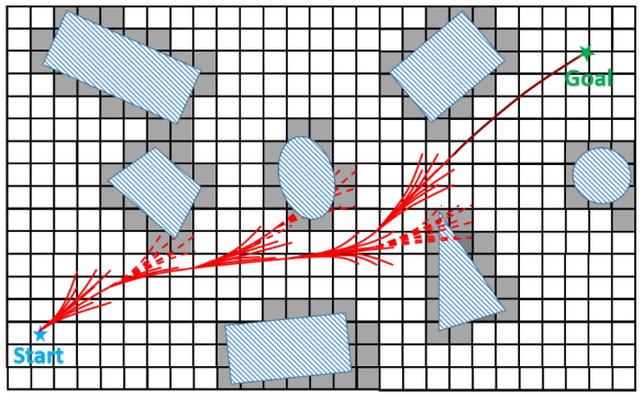
B-spline Trajectory Optimization
- Drawback of the kinodynamic path searching:
- The path produced by the
kinodynamic path searchingcan besuboptimal. - The path is often
close to obstaclesince distance information in the free space is ignored.
- The path produced by the
- Improve the smoothness and clearance of the path via
B-spline optimization.- Utilize the
convex hull propertyof uniform B-splines. - Incorporate
gradient informationfrom the Euclidean distance field and dynamic constraints. - It
convergeswithin a very short duration to generate smooth, safe and dynamically feasible trajectories.
- Utilize the
Uniform B-splines
- A B-spline is a
piecewise polynomialuniquely determined by its degree \(p_b\). - Control points: \(\{ \mathbf{Q}_0, \mathbf{Q}_1, \cdots, \mathbf{Q}_N \}, \mathbf{Q}_i \in \mathbb{R}^3\).
- Knot vector: \([t_0, t_1, \cdots, t_M], M = N + p_b + 1, t_m \in \mathbb{R}\).
- For a uniform B-spline, each knot span \(\Delta t_m = t_{m+1} - t_m\) has identical value \(\Delta t\).
- A B-spline trajectory is parameterized by time \(t \in [t_{p_b}, t_{M-p_b}]\).
- The derivative of a B-spline is also a B-spline.
To evaluate the position at time \(t \in [t_m, t_{m+1}) \subset [t_{p_b}, t_{M-p_b}]\), normalize \(t\) as:
\[s(t) = \frac{t-t_m}{\Delta t}.\]Then, the position can be evaluated using the matrix representation:
where \(\mathbf{M}_{p_b+1}\) is a constant matrix determined by \(p_b = 3\).
Convex Hull Property
- This property is extremely useful for ensuring the
dynamic feasibility and safetyof the entire trajectory. - Dynamic feasibility:
- It suffices to constrain all velocity and acceleration control points.
- velocity: \(\{ \mathbf{V}_0, \mathbf{V}_1, \cdots, \mathbf{V}_{N-1} \}, \mathbf{V}_i = \frac{1}{\Delta t} (\mathbf{Q}_{i+1} - \mathbf{Q}_i), \mathbf{V}_i \in [-v_{max}, v_{max}]^3\).
- acceleration: \(\{ \mathbf{A}_0, \mathbf{A}_1, \cdots, \mathbf{A}_{N-2} \}, \mathbf{A}_i = \frac{1}{\Delta t} (\mathbf{V}_{t+1} - \mathbf{V}_i), \mathbf{A}_i \in [-a_{max},a_{max}]^3\).
- It suffices to constrain all velocity and acceleration control points.
-
Safety:
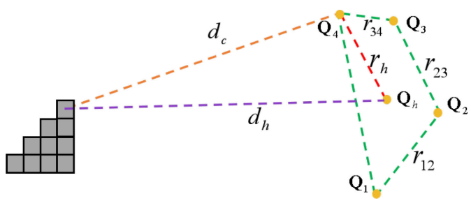
- Need to ensure that all its convex hulls are
collision-free.- The distance between
any one occupied voxelandany one point\(Q_h\) in the convex hull \(d_h > 0\). - \(d_h > d_c - r_h\).
- \(d_c\): the distance between the
voxeland any onecontrol point. - \(r_h \le r_{12}+r_{23}+r_{34}\).
- Then, \(d_h > d_c - (r_{12}+r_{23}+r_{34})\).
- \(d_c\): the distance between the
- The distance between
- Need to ensure that all its convex hulls are
Thus, the convex hull is guaranteed to be collision-free if we ensure:
\[d_c > 0, \quad r_{j,j+1} < d_c/3, \quad j \in \{ 1,2,3 \}.\]Cost Function
- For a B-spline trajectory:
- Degree: \(p_b\).
- Control points: \(\{ Q_0, Q_1, \cdots, Q_N \}\).
- Optimize the subset of \(N+1-2p_b\) control points: \(\{ Q_{p_b}, Q_{p_b+1}, \cdots, Q_{N-p_b} \}\).
- The first and last \(p_b\) control points should not be changed because they determine the
boundary state.
Define the overall cost function as:
\[f_{total} = \lambda_1 f_s + \lambda_2 f_c + \lambda_3(f_v + f_a),\]where
- \(f_s\): smoothness cost.
- \(f_c\): collision cost.
- \(f_v\): soft limit on velocity.
- \(f_a\): soft limit on acceleration.
- \(\lambda_1,\lambda_2,\lambda_3\): trade off the
smoothness,safety, anddynamic feasibility.
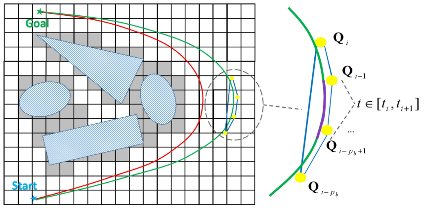
Smoothness cost \(f_s\):
- captures the
geometric informationof the trajectory. - does not depend on time allocation.
- because that after optimization the time allocation may be adjusted.
Define \(f_s\) via using an elastic band cost function:
\[f_s = \sum_{i = p_b-1}^{N-p_b+1}\Vert \underbrace{(Q_{i+1} - Q_i)}_{F_{i+1,i}} + \underbrace{(Q_{i-1} - Q_i)}_{F_{i-1,i}} \Vert^2.\]From a physical standpoint:
- view a trajectory as an elastic band.
- \(F_{i+1,i}\) and \(F_{i-1,i}\) are the joint force of two springs connecting the nodes \(Q_{t+1},Q_i\) and \(Q_{i-1},Q_i\), respectively.
- If all terms equal to zero, all the control points would uniform distribute in a straight line, which is ideally smooth.
Collision cost \(f_c\):
- Formulate as the repulsive force of the obstacles acting on each control point.
where
- \(d(Q_i)\) is the distance between \(Q_i\) and the closet obstacle.
- \(F_c()\) is a differentiable potential cost function.
- \(d_{thr}\) specifying the threshold of obstacle clearance.
Also, the following euqation must be satisfied so that the trajectory is collision-free:
\[d_c > 0, \quad r_{j,j+1} < d_c/3, \quad j \in \{ 1,2,3 \}.\]- \(d_c > 0\) is apparent.
- In practice, select small \(r_{j,j+1} < 0.2\), the trajectory is safe in most cases.
- This may be invalid in extreme cases:
- the environment is very cluttered.
- in this case, select smaller \(r_{j,j+1}\), the trajectory also can be safe.
Dynamic feasibility cost:
- penalize velocity or acceleration along the trajectory exceeding maximum allowable value \(v_{max},a_{max}\).
The penalty for \(v_\mu\) is:
\[F_v(v_\mu) = \begin{cases} (v_\mu^2 - v_{max}^2)^2 & v_\mu^2 > v_{max}^2 \\ 0 & v_\mu^2 \le v_{max}^2, \end{cases}\]where \(\mu \in \{x,y,z\}\).
Then, the dynamic feasibility cost function is defined as:
\[\begin{aligned} f_v & = \sum_{\mu}\sum_{i=p_b-1}^{N-p_b} F_v(V_{i\mu}), \\ f_a & = \sum_{\mu}\sum_{i=p_b-2}^{N-p_b} F_a(A_{i\mu}). \end{aligned}\]Time Adjustment
- We have constrained kinodynamic feasibility in the path searching and optimization.
- However, sometimes we get
infeasible trajectories. Reason:- gradient information tends to
lengthen the overall trajectorywhile pushing it far from obstacles. - Then, the quadrotor
has to fly more aggressivelyin order to travel longer distance within the same time. - Unavoidably causes
over aggressive motionif the original motion is already near to the physical limits.
- gradient information tends to
- To guarantee dynamic feasibility:
- adopt a
time adjustmentmethod.- based on the relations between the
derivatives control pointsand thetime allocationof the non-uniform B-spline.
- based on the relations between the
- Change the flight aggressiveness as we expected by
adjustingthe associated time allocation (knot spans). - Thus, the dynamic feasibility can be ensured
without over-conservative constraints.
- adopt a
Non-Uniform B-spline
- A more general kind of B-spline.
- Difference to uniform B-spline:
- Each of its knot span \(\Delta t_m = t_{m+1}-t_m\) is independent to others.
Knot Spans Adjustment
Let \(\mathbf{V}_i' = [V_{i,x}', V_{i,y}', V_{i,z}']^T\) be an infeasible control point of velocity.
Let \(V_{i,\mu}'\) be the largest infrasible component and \(\vert V_{i,\mu}' \vert = v_m\).
\(V_{i,\mu}'\) is influenced by the duration \((t_{i+p_b+1} - t_{i+1})\).
If we change the duration as follows:
\[\hat{t}_{i+p_b+1} - \hat{t}_{i+1} = \mu_v(t_{i+p_b+1} - t_{i+1}),\]where \(\mu_v = \frac{v_m}{v_{max}}\).
Then, the velocity is feasible as:
\[\hat{V}_{i,\mu} = \frac{p_b(Q_{i+1,\mu} - Q_{i,\mu})}{\hat{t}_{i+p_b+1} - \hat{t}_{i+1}} = \frac{1}{\mu_v}V_{i,\mu}' = v_{max}.\]Similarly, let \(\mu_a = \left( \frac{a_m}{a_{max}} \right)^{\frac{1}{2}}\), then,
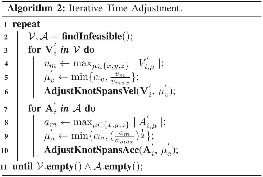
\[\hat{A}_{i,\mu} = \frac{1}{\mu_a^2}A_{i,\mu}' = a_{max}.\]Iterative Time Adjustment
- It iteratively finds the infeasible velocity and acceleration control points of the trajectory.
- Adjust the corresponding
knot spans.- Bounding \(\mu_v', \mu_a'\) with two constant \(\alpha_v,\alpha_a\) slightly larger than \(1\), prevents any time span from being extended excessively.
Experiment
- C++, NLopt (a general non-linear optimization solver).
- Parameters:
- Path searching: \(\gamma = 2, \tau = 0.5\).
- Optimization: \(\lambda_1 = 10.0, \lambda_2 = 0.8, \lambda_3 = 0.01\).
- Time adjustment: \(\alpha_v = \alpha_a = 1.1\).
- Platforms:
- Autonomous flight quadrotor:
- Velodyne VLP-16 3D LiDAR. LOAM.
- estimate the pose of the quadrotor.
- generate a dense point cloud map.
- Fuse the laser-based estimation with IMU and sonar measurements by EKF.
- Intel i7-5500U, 8G RAM, 256G SSD.
- motion planning.
- state estimation.
- mapping.
- control.
- Velodyne VLP-16 3D LiDAR. LOAM.
- Fast-replanning quadrotor:
- light-weight and agile.
- OptiTrack.
- Nvidia TX2.
- motion planning.
- control.
- Autonomous flight quadrotor:
- Experiments:
- Fast autonomous flight in unknown cluttered environments.
- Fast-replanning capability in aggressive flight.
- Re-Planning Strategy:
- The quadrotor has to re-plan its trajectory frequently in an unknown environment due to the limited sensing range.
- Receding-Horizon local planning:
- Trajectories are generated only within the known space.
- The path searching is terminated once a motion primitive ends outside the range.
- Then, followed by the optimization and time adjustment.
- Re-planning triggering mechanism:
- If the current trajectory collides with newly emergent obstacle.
- The planner is called at fixed intervals of time.
References
- B. Zhou, F. Gao, L. Wang, C. Liu, and S. Shen, “Robust and Efficient Quadrotor Trajectory Generation for Fast Autonomous Flight,” IEEE RA-L, 2019.
-
D. Dolgov, S. Thrun, M. Montemerlo, and J. Diebel, “Path planning for autonomous vehicles in unknown semi-structured environments,” IJRR, vol. 29, no. 5, pp. 485–501, 2010. ↩