Robust Deep RL Against Adversarial Perturbations on State Observations
Motivation
- DRL has achieved great success on some safety-critical applications, such as autonomous driving.
- The existence of adversarial examples in DNNs and many successful attacks to DRL motivates us to study robust DRL algorithms.
- Problems in state observation:
- May contain
uncertaintythat naturally originates from unavoidable sensor measurement errors or equipment inaccuracy. - Adversarial noises.
- May contain
- Since the observations deviate from the true states:
- They can mislead the agent into making
suboptimal actions. - A policy not robust to such uncertainty can lead to
catastrophic failures.
- They can mislead the agent into making
- Existing works:
- have limited success.
- lack for theoretical principles.
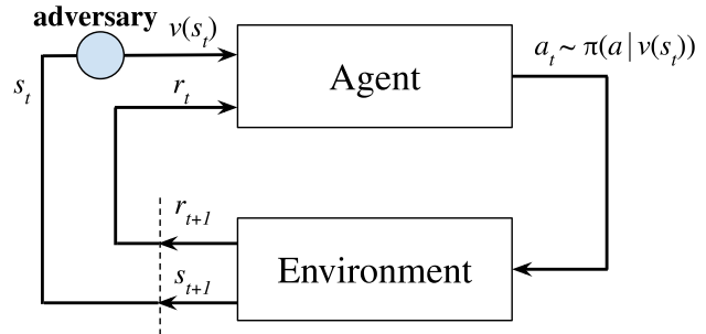
- To ensure safety under the worst case uncertainty, consider the
adversarial setting:- The observation is adversarially perturbed from \(s\) to \(v(s)\).
- The underlying true environment state \(s\) where the agent locates is unchanged.
- This setting is aligned with many adversarial attacks on state observations.
- To improve robustness under this setting:
- Extend existing adversarial defenses for supervised learning (adversarial training).
- Attack the agent and generate trajectories adversarially dyring training time, and apply any existing DRL algorithm to hopefully obtain a robust policy.
- Drawback:
- For most environments, naive adversarial training can make training
unstableanddeteriorate agent performance. - Does not significantly improve robustness
under strong attacks.
- For most environments, naive adversarial training can make training
- DRL agents can be brittle even without any adversarial attacks,
only with a small noise:- An agent may fail occasionally but catastrophically during regular rollouts.
- A small noise added to the environment may lead the agent to low reward.
- In practical applications, such a small noise can be naturally prevalent.
- Thus, prohibit the use of DRL in safety critical domains (autonomous driving).
- Related Work:
- Robust RL:
- Each element of RL can contain
uncertainty:- Observation.
- More suitable to model worst case errors in observation process (sensro errors and equipment inaccuracy).
- Action.
- Transition dynamics.
- Reward.
- Observation.
- Each element of RL can contain
Adversarial attackson state observations:- FGSM based attack.
- on pixel space.
- Black-box attacks.
- Multi-step gradient based attacks.
- FGSM based attack.
- Robust RL:
Contributions
- Formulate the perturbation on state observations as a modified MDP, called state-adversarial Markov Decision Process (
SA-MDP).- Study its fundamental properties.
- Based on the theory of SA-MDP, propose a theoretically principled
robust policy regularizer.- Related to the
total variation (TV) distanceorKL-divergenceon perturbed policies.
- Related to the
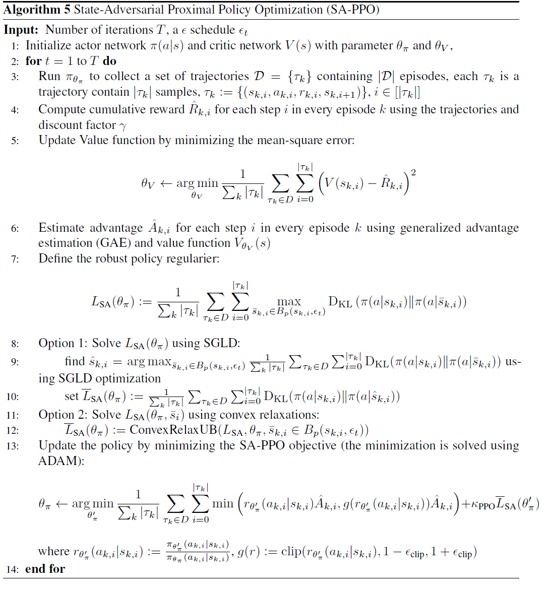
- Develop a theoretically principled
policy regularizationwhich can be applied to a large family of DRL algorithms.- PPO.
- DDPG.
- DQN.
- Improve the
robustnessof PPO, DDPG, and DQN agents under a suite ofstrong white box adversarial attackson state observations.- The robust SARSA attack (RS attack).
- Maximal action difference attack (MAD attack).
- Robust policy noticeably improves DRL performance even without an adversary in a number of environments.
- Code.
Method
SA-MDP
Definition
Adversary: \(v(s): S \to S\).- Perturb the observation of the agent.
- The worst case noise in measurement.
- State estimation uncertainty.
- Assumption:
- Stationary, Deterministic and Markovian Adversary.
- \(v(s)\) is a deterministic function.
- Only depend on the current state \(s\).
- Does not change over time.
- This assumption holds for many adversarial attacks.
- Restrict the power of the adversary:
- Define perturbation set \(B(s)\).
- \(B(s)\) is a set of states, \(s \in B(s)\).
- Usually defined as an \(L_\infty\) norm ball around \(s\) with a radius \(\epsilon\): \(B(s) = \{s_v : \lVert s - s_v \rVert_\infty \le \epsilon\}\).
- \(\epsilon\) is also referred to as the
perturbation budget.
- Contain all allowed perturbations of the adversary \(v(s) \in B(s)\).
- \(B(s)\) is usually a set of task-specific neighbouring states of \(s\).
- Bound sensor measurement errors.
- The observation still meaningful even with perturbations.
- \(B(s)\) is a set of states, \(s \in B(s)\).
- Restrict the adversary to perturb a state \(s\) only to a predefined set of states.
- Define perturbation set \(B(s)\).
- Perturb the observation of the agent.
Action: \(\pi(a \vert v(s))\).- may be sub-optimal.
- Thus, the adversary is able to reduce the reward.
Next state: \(s\), not \(v(s)\).
Bellman Equations
Define the adversarial value function as follows:
Action-value function:
Bellman equations for fixed \(\pi\) and \(v\):
Find the value functions under optimal (strongest) adversary \(v^\star(\pi)\):
- Minimize the total expected reward for a
fixed policy\(\pi\).
Define the optimal adversarial value and action-value functions as:
Bellman contraction for optimal adverasry:
- Similar to the policy evaluation procedure in regular MDP.
- In the same spirit as Bellman optimality equations.
Find an optimal policy \(\pi^\star\) under the strongest adversary \(v^\star(\pi)\) in the SA-MDP setting:
Theorem: There exists an SA-MDP and some stochastic policy \(\pi \in \Pi_{MR}\) such that we cannot find a better deterministic policy \(\pi' \in \Pi_{MD}\) satisfying \(V_{\pi',v*(\pi')}(s) \ge V_{\pi,v*(\pi)}(s)\) for all \(s\in S\).
- Some stochastic policies are better than any other deterministic policies in SA-MDP.
- Contrarily, in a regular MDP, for any stochastic policy, we can find a deterministic policy that is at least as good as the stochastic one.
- Even looking for both deterministic and stochastic policies, we cannot always find an optimal one.
- Under the optimal \(v^\star\), an optimal policy \(\pi^\star \in \Pi_{MR}\) does not always exist for SA-MDP.
- Therefore, it is
diffcult to find an optimal policy under the optimal adversary.
Despite that, under certain assumptions, the loss in performance due to an optimal adversary can be bounded:
- If the differences between the action distributions under state perturbations are not too large, the performance gap between \(V_{\pi,v*(\pi)}(s)\) and \(V_\pi(s)\) can be bounded.
- Regularize \(D_{TV}\) during training can obtain a policy that is robust under strong adversaries.
- A bounded state perturbation \(s_v\) produces bounded \(D_{TV}\).
where \(\alpha\) is a constant that does not depend on \(\pi\):
\[\alpha = 2\left[ 1 + \frac{\gamma}{(1-\gamma)^2} \right] \max_{(s,a,s')\in S\times A \times S}\lvert R(s,a,s')\rvert.\]SA-MDP on PPO
- Stochastic policies.
The total variation distance is not easy to compute for most distributions, so we upper bound it again by KL-divergence:
Define the policies as multivariate Gaussian distribution:
The KL-divergence can be given as:
\[D_{KL}(\pi(a\vert s),\pi(a\vert s_v)) = \frac{1}{2} \left( \log\lvert\Sigma_{s_v}\Sigma_s^{-1}\rvert +tr(\Sigma_{s_v}^{-1}\Sigma_s) + (\mu_{s_v} - \mu_s)^T \Sigma_{s_v}^{-1}(\mu_{s_v} - \mu_s) - \lvert A \rvert \right),\]where
- The mean terms \(\mu_s,\mu_{s_v}\) are produced by neural networks \(\mu_{\theta}(s), \mu_{\theta}(s_v)\).
- \(\Sigma = \Sigma_{s_v} = \Sigma_s\) is a diagonal matrix independent of state \(s\).
Regularize KL-divergence for all \(s_v \in B(s)\):
- Lead to a smaller upper bound of the loss in performance.
- Directly related to agent performance under optimal adversary.
- Ignore constant terms, then, the following
robust policy regularizercan be obtained:
- Replace \(\max_{s\in S}\) term with a more practical and optimizer-friendly
summationover all states in sampled trajectory.
Minimizing the above equation is challenging as it is a minimax objective.
- Because \(\nabla_{s_v} \mathcal{L}(s_v,\theta_\mu)\vert_{s_v = s} = 0\), so using gradient descent directly cannot solve the inner maximization problem.
- Propose two first order approaches to sovle it:
- Convex relaxation based method.
- Enable an efficient analysis of the outer bounds for a neural network.
- Leverage it as a generic optimization tool for solving minimax functions involving neural networks.
- We can obtain an
upper boundfor \(\mathcal{L}_s(s_v,\theta_\mu): \bar{\mathcal{L}}_s(\theta_\mu) \ge \mathcal{L}_s(s_v,\theta_\mu)\) for all \(s_v\in B(s)\). - Compute \(\bar{\mathcal{L}}_s(\theta_\mu)\) is only a constant factor slower than compute \(\mathcal{L}_s(s,\theta_\mu)\) when an efficient relaxation is used.
- Stochastic Gradient Langevin Dynamics (SGLD) based solver.
- Convex relaxation based method.
Then, the minimization problem can be solved by:
\[\min_{\theta_\mu}\frac{1}{2}\sum_s \bar{\mathcal{L}}_s(\theta_\mu) \ge \min_{\theta_\mu}\frac{1}{2}\sum_s\max_{s_v\in B(s)}\mathcal{L}_s(s_v,\theta_\mu) = \min_{\theta_\mu}\mathcal{L}_{PPO}(\theta_\mu).\]Then, we can add \(\mathcal{L}_{PPO}\) as part of the policy optimization objective, and solve PPO using SGD as usual.
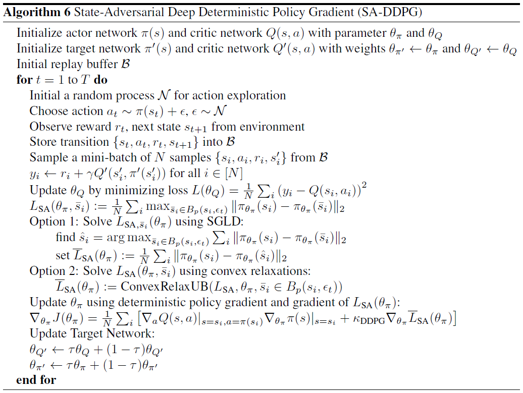
SA-MDP on DDPG
- Deterministic policy.
The total variation distance \(D_{TV}(\pi(\cdot\vert s), \pi(\cdot\vert s_v))\) is malformed.
- The densities at different states \(s\) and \(s_v\) are very likely to be completely non-overlapping.
To adress this issue:
- Define a smoothed version of policy \(\bar{\pi}(a\vert s)\).
- Add independent
Gaussian noisewith variance \(\sigma^2\) to each action: \(\bar{\pi}(a\vert s)\sim N(\pi(s),\sigma^2 I_{\lvert A \rvert})\).
- Add independent
Then, the total variation distance can be computed by:
where \(d = \lVert \pi(s) - \pi(s_v)\rVert_2\).
Then, if we can penalize \(\sqrt{\frac{2}{\pi}}\frac{d}{\sigma}\), \(D_{TV}\) can be bounded.
Define the robust policy regularizer for DDPG as:
- For each state in a sampled batch of states, we need to solve a maximization problem:
- Using SGLD.
- Convex relaxation.
Then, during training time our goal is to keep \(\mathcal{L}_{DDPG}\) small.
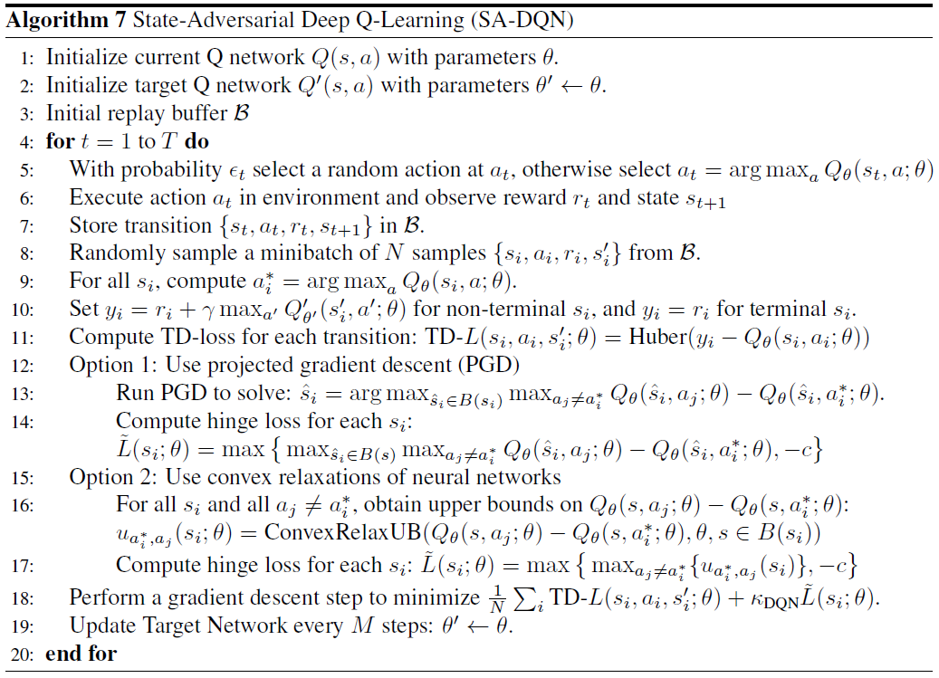
SA-MDP on DQN
- The action space is finite.
- The deterministic action is determined by the maximum \(Q\) value.
- \(\pi(a\vert s) = 1\), when \(a = \arg\max_{a'}Q(s,a')\).
- \(\pi(a\vert s) = 0\), otherwise.
Then, the total variation distance is:
- We want to make the top-1 action stay unchanged after perturbation.
Define the robust policy regularizer as:
where \(a^\star(s) = \arg\max_a Q_\theta(s,a)\) and \(c\) is a small positive constant.
- The sum is over all \(s\) in a sampled batch.
- It is more similar to the robustness of classification tasks.
- Treat \(a^\star(s)\) as the
correctlabel.
- Treat \(a^\star(s)\) as the
- The maximization can be solved using:
- Projected Gradient Descent (PGD).
- Convex relaxation of neural networks.
Then, add \(\mathcal{L}_{DQN}\) as part of the optimization objective.
Adversarial Attacks under Assumption
- Discuss a few strong adversarial attacks under assumption.
- Propose two novel
critic independentattacks for DDPG and PPO:- Robust SARSA (RS) attack.
- Maximal Action Difference (MAD) attack.
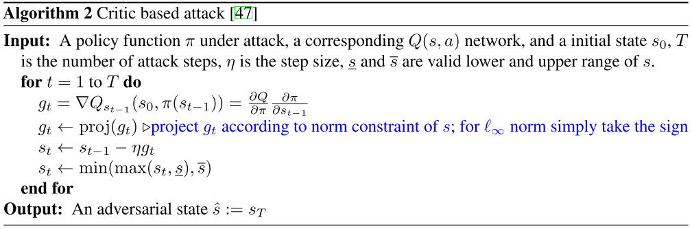
Critic based attack
Many works use the gradient of \(Q(s,a)\) to provide the direction to update states adversarially in \(K\) steps:
Define the adversarial state as: \(s_v = s^{K-1}\).
\[s^{k+1} = s^k - \eta \cdot proj[\nabla_{s^k}Q(s^0,\pi(s^k))], \quad k=0,\cdots,K-1.\]Where
- \(proj[\cdot]\) is a projection to \(B(s)\).
- \(\eta\) is the learning rate.
- \(s^0\) is the state under attack.
It attempts to find a state \(s_v\) triggering an action \(\pi(s_v)\) minimizing the action-value at state \(s^0\).
- Require a \(Q\) function to find the best perturbed state \(s_v\).
This attack has a few drawbacks:
- Attack strength strongly depends on
critic quality.- If \(Q\) is poorly learned, the attack fails as no correct update direction is given.
- Not robust against small perturbations.
- Has obfuscated gradients.
- If \(Q\) is poorly learned, the attack fails as no correct update direction is given.
- It relies on \(Q\) function which is specific to the training process.
- Not applicable to many actor-critic methods (TRPO, PPO) using a learned value function \(V(s)\) instead of \(Q\).
- \(V(s_v)\) represents the value of \(s_v\) rather than the value of taking \(\pi(s_v)\) at \(s^0\).
- \(V(s_v) = \max_a Q(s_v,a) \neq \max_a Q(s^0,a)\).
- \(V(s_v)\) represents the value of \(s_v\) rather than the value of taking \(\pi(s_v)\) at \(s^0\).
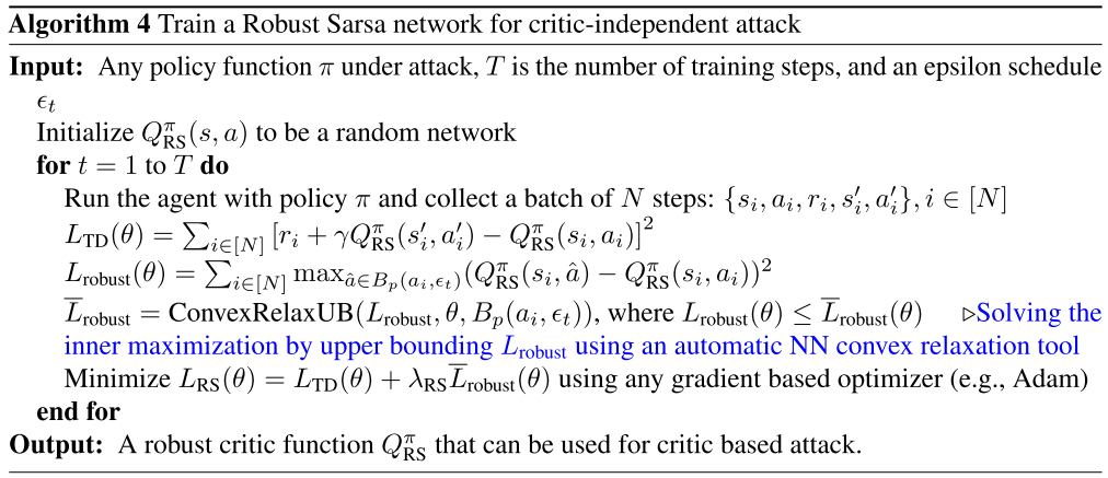
Robust SARSA (RS) attack
Since \(\pi\) is fixed during evaluation:
- We can learn its corresponding \(Q^\pi(s,a)\) using on-policy TD algorithms without knowing the critic network used during training.
- The robustness of \(Q^\pi(s,a)\) is very important.
- If it is
not robustagainst small perturbations:- Given a state \(s_0\), a small change in \(a\) will significantly reduce \(Q^\pi(s_0,a)\), which does not reflect the true action-value.
- It cannot provide a good direction for attacks.
- If it is
Use the on-policy TD-learning algorithm (SARSA) to learn \(Q^\pi(s,a)\) with an additional robustness objective to minimize:
\[L_{RS}(\theta) = \sum_{i\in [N]}\left[ r_i + \gamma Q_{RS}^\pi(s_i',a_i') - Q_{RS}^\pi(s_i,a_i) \right]^2 + \lambda_{RS} \sum_{i\in [N]}\max_{\hat{a}\in B(a_i)}(Q_{RS}^\pi(s_i,\hat{a}) - Q_{RS}^\pi(s_i,a_i))^2,\]where
- The first summation is the TD-loss.
- The second summation is the robustness penalty with regularization \(\lambda_{RS}\).
- \(N\) is the batch size and each batch contains N tuples of transitions \((s,a,r,s',a')\) sampled from agent rollouts.
- \(B(a_i)\) is a small set near action \(a_i\).
- The inner maximization can be solved using convex relaxation of neural networks.
- Use \(Q_{RS}^\pi\) to perform critic-based attacks.
The attack strength of this attack does not depend on the quality of an existing critic.
Maximal Action Difference (MAD) attack
- An effective attack, does not depend on a critic.
- Find an adversarial state \(s_v\) by maximizing \(D_{KL}(\pi(\cdot\vert s),\pi(\cdot\vert s_v))\).
Let
\[L_{MAD}(s_v) = - D_{KL}(\pi(\cdot\vert s),\pi(\cdot\vert s_v)).\]Then, find \(s_v\) by:
\[\begin{aligned} \arg\min_{s_v \in B(s)} L_{MAD}(s_v) & = \arg\max_{s_v\in B(s)} D_{KL}(\pi(\cdot\vert s),\pi(\cdot\vert s_v)) \\ & = \arg\max_{s_v\in B(s)} (\pi_\theta(s) - \pi_\theta(s_v))^T\Sigma^{-1}(\pi_\theta(s) - \pi_\theta(s_v)). \end{aligned}\]The objective can be optimized using SGLD to find a good \(s_v\).
For DDPG, set \(\Sigma = I\).

References
- H. Zhang, H. Chen, C. Xiao, B. Li, D. Boning, and C. J. Hsieh, “Robust deep reinforcement learning against adversarial perturbations on state observations,” Neural Information Processing Systems, 2020.