Robust RL on State Observations with Learned Optimal Adversary
Motivation
- Adversarial attacks used in image classificant tasks.
- Attacks:
- Add imperceptible noises into the observations of states.
- The observed environment slightly differs from true environment states.
- Add imperceptible noises into the observations of states.
- Using RL in
safety-crucialapplications:- Autonomous driving.
- It is important for real-world RL agent
under unpredictable sensing noise. - Contribute to the
reality gap:- An agent working well in simulated environments may fail in real environments due to
noises in observations.
- An agent working well in simulated environments may fail in real environments due to
- The
weaknessof a DRL agent on the perturbations of state observations:- Vulnerability in function approximators.
- Originate from the highly non-linear and blackbox nature of neural networks.
Example: For Atari games, CNN extracts features (e.g. for game of Pong, the position and velocity of the ball) from input frames. Using attacks to add noises in the observations, CNN will extract wrong features.
- Intrinsic weakness of policy.
- Even perfect features for states are extracted, a policy can still make mistakes due to an intrinsic weakness.
Example: In a finite-state MDP, there is no function approximation error, but the agent can still be vulnerable to small perturbations on observations (e.g. perturb the observation to one of the neighbors of the true states).
- Vulnerability in function approximators.
- To improve the
robustnessof RL:- A more robust function approximator.
- Add a robust policy regularizer to the loss function. (indistinctive)
- A policy aware of perturbations on observations.
- A more robust function approximator.
- Related works:
- SA-MDP
- The
true statein the environment is not perturbed by the adversary. Example: GPS sensor readings on a car are naturally noisy, but the ground truth location of the car is not affected by the noise.
- The
- Robust MDP (RMDP)
- The worst case
transition probabilitiesof the environment are considered. - This setting is essentially different from SA-MDP.
- The worst case
- Robust Adversarial RL (RARL)
- Learn an adversary online together with an agent.
- Train an agent and an adversary under the two-player Markov game setting.
- The adversary can change the environment states through actions directly applied to environment.
- The goal is to improve the robustness against
environment parameter changes, such as mass, length, or friction.
- Action Robust RL
- The learning process of above works are still a
MDP, but consider the perturbations on state observations will lead it to aPOMDPproblem.
- SA-MDP
Contributions
- With a fixed agent policy:
- An optimal adversary to perturb state observations can be found.
- The learned adversary is much stronger than previous ones.
- And, it is guaranteed to obtain worst case agent reward.
- An optimal adversary to perturb state observations can be found.
- Propose a framework of alternating training with learned adversaries (ATLA).
- Training an adversary online together with the agent using policy gradient following the optimal adversarial attack framework.
- Improve the robustness of the agent.
History(the past states and actions) can be important for learning a robust agent.- Propose to use a
LSTMbased policy in the ATLA framework.- It is
more robustthan policy parameterized as regular feedforward NNs.
- It is
- Propose to use a
Method
POMDP
\[\langle S,A,O,\Omega,R,P,\gamma \rangle\]- \(O\) is a set of observations.
- \(\Omega\) is a set of conditional observation probabilities \(p(o\vert s)\).
- POMDP typically require history-dependent optimal policies.
- A history-dependent policy is defined as \(\pi: H\to P(A)\).
- \(H\) is the set of history.
- History \(h_t\) at time \(t\) is denoted as \((s_0,a_0,\cdots,s_{t-1},s_{t-1},s_t)\).
SA-MDP
- \(\langle S,A,B,R,P,\gamma \rangle\).
- \(B\) is a mapping from a state \(s\in S\) to a set of states \(B(s)\in S\).
- \(B\) limits the power of adversary: \(v(s)\in B(s)\).
Goal: solve an optimal policy \(\pi^\star\) under the optimal adversary \(v^\star(\pi^\star)\).- The
related workdid not give an explicit algorithm to solve SA-MDP and found that a stationary optimal policy need not exist.
Find the optimal adversary under a fixed policy
- The optimal adversary leads to the worst case performance under bounded perturbation set \(B\).
- An absolute lower bound of the excepted cumulative reward an agent can receive.
- The adversary’s goal is to
reduce the reward earned by the agent.
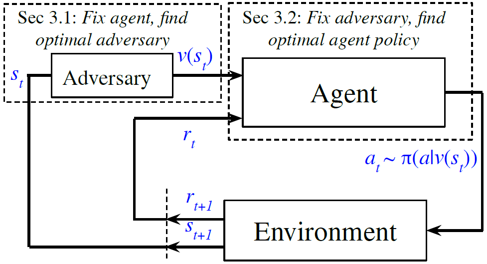
Solving the optimal adversary \(v^\star(s)\) (policy) in MDP setting:
Environment dynamics:- Merge the two parts into a MDP:
- A fixed and stationary agent policy \(a = \pi(s_v)\), where \(s_v = proj_{B(s)} (s + \Delta)\).
- The original environment dynamics \(s' = P(s,a)\).
- Merge the two parts into a MDP:
State: \(s\), the true state.Action: \(\Delta = v(s)\).Reward: a weighted average of \(-R\).
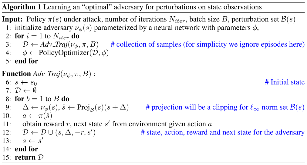
Parameterize the adversary as a neural network function:
- Using any popular DRL algorithm to learn an optimal adversary.
- No existing adversarial attacks follow such a theoretically guided framework.
The algorithm is shown as follows:
Advantages:
- The learned adversary is strong.
- Rather than using any heuristic to generate a perturbation.
- The previous strong attack (RS attack) can successful fail an agent and make it stop moving and receive a small positive reward.
- While, the learned attack can trick the agent into
moving toward the opposite directionof the goal and receive alarge negative reward.
- Keep improving the adversary with a goal of receiving as less reward as possible.
- The learned adversary requires no gradient access to the policy.
- Previous attacks are mostly gradient based approach and need to access the values or gradients to a policy or value function.
Find the optimal policy under a fixed adversary
- Based on POMDP \(\langle S,A,O,\Omega,R,P,\gamma \rangle\):
- \(O = \bigcup_{s\in S}\{ s'\vert s'\in supp(v(\cdot\vert s)) \}\).
- \(P(o_t = s' \vert s_t = s) = v(s_v = s' \vert s_t = s)\).
- Using recurrent policy gradient theorem on POMDPs.
- Using LSTM as function approximators for the value and policy networks.
For PPO, use the loss function:
\[L(\theta) = \mathbb{E}_{h_t}\left[\min\left[ \frac{\pi_\theta(a_t\vert h_t)}{\pi_{\theta_{old}}(a_t\vert h_t)} A_{h_t}, clip\left(\frac{\pi_\theta(a_t\vert h_t)}{\pi_{\theta_{old}}(a_t\vert h_t)}, 1-\epsilon,1+\epsilon\right)A_{h_t} \right]\right],\]where
- \(h_t = \{ s_v^0, a_0, \cdots, s_v^t \}\) contains all history of
perturbed statesandactions. - \(A_{h_t}\) is a baseline advantage function modeled using a LSTM.
Alternating training with learned adversaries (ATLA)
- Training an adversary online with the agent:
- First keep the agent fixed, optimize the adversary (parameters of NN).
- Then keep the adversary fixed, optimize the agent.
- Both adversary and agent can be updated using PPO.
Algorithm:
- Using a strong and learned adversary that tries to
find intrinsic weakness of the policy. - To obtain a good reward, the policy must learn to defeat such an adversary.
- Using \(s\) instead of \(s_v\) to train the advantage function and policy of the agent leads to worse performance.
- It does not follow the theoretical framework of SA-MDP.

References
- Robust Reinforcement Learning on State Observations with Learned Optimal Adversary, under review at ICLR, 2021.